The new*() constructors, and the system around them
An energyRt model is a set of objects, each built by a new*() function.
Commodities — the things that flow
newCommodity()Processes — the things that move or transform them
newSupply(), newImport(), newExport()newDemand()newTechnology()newStorage(), newTrade()Containers — how they are assembled
newRepository() — a bag of objectsnewHorizon() — the yearsnewModel() — objects + regions + horizonPolicy (later chapters)
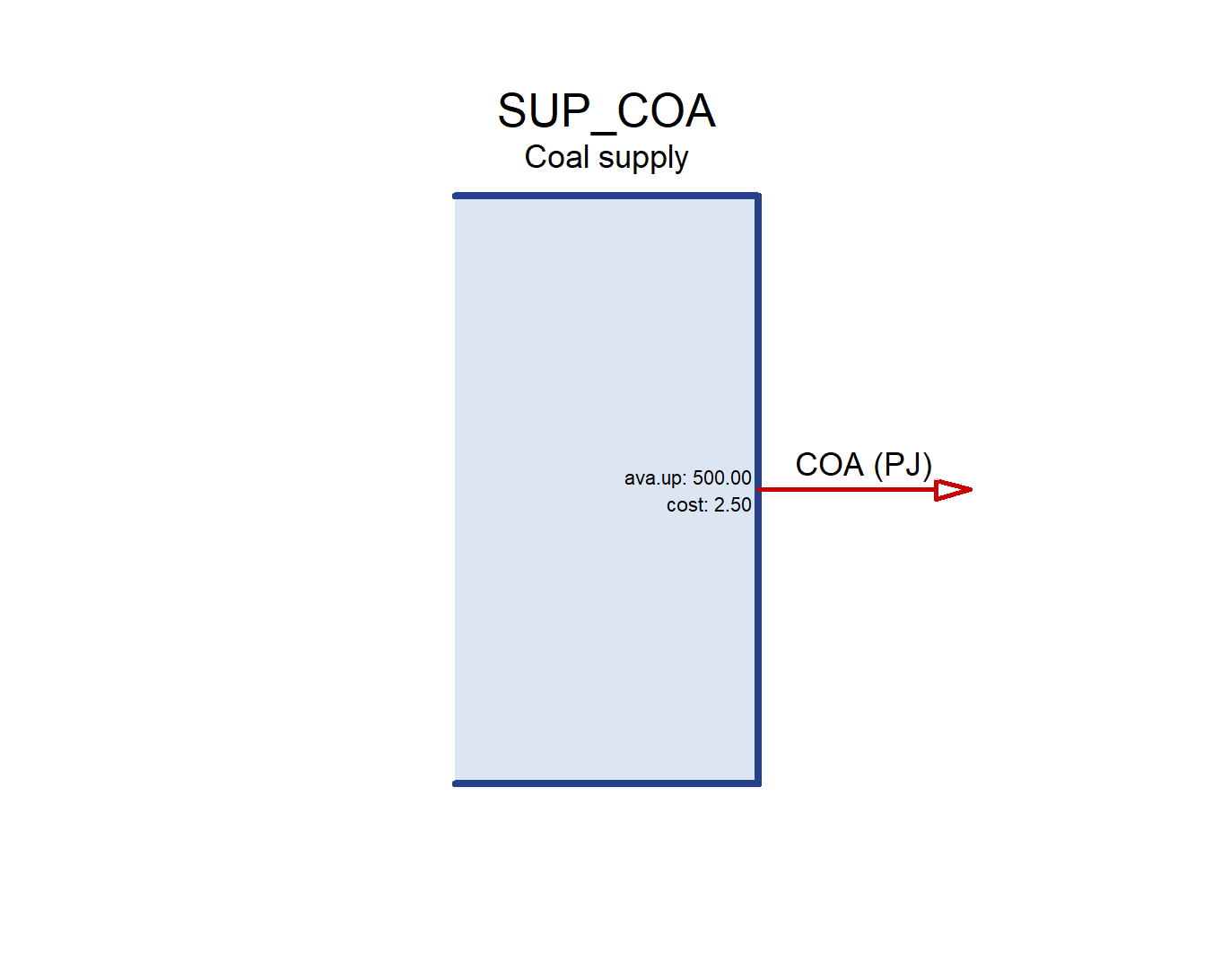
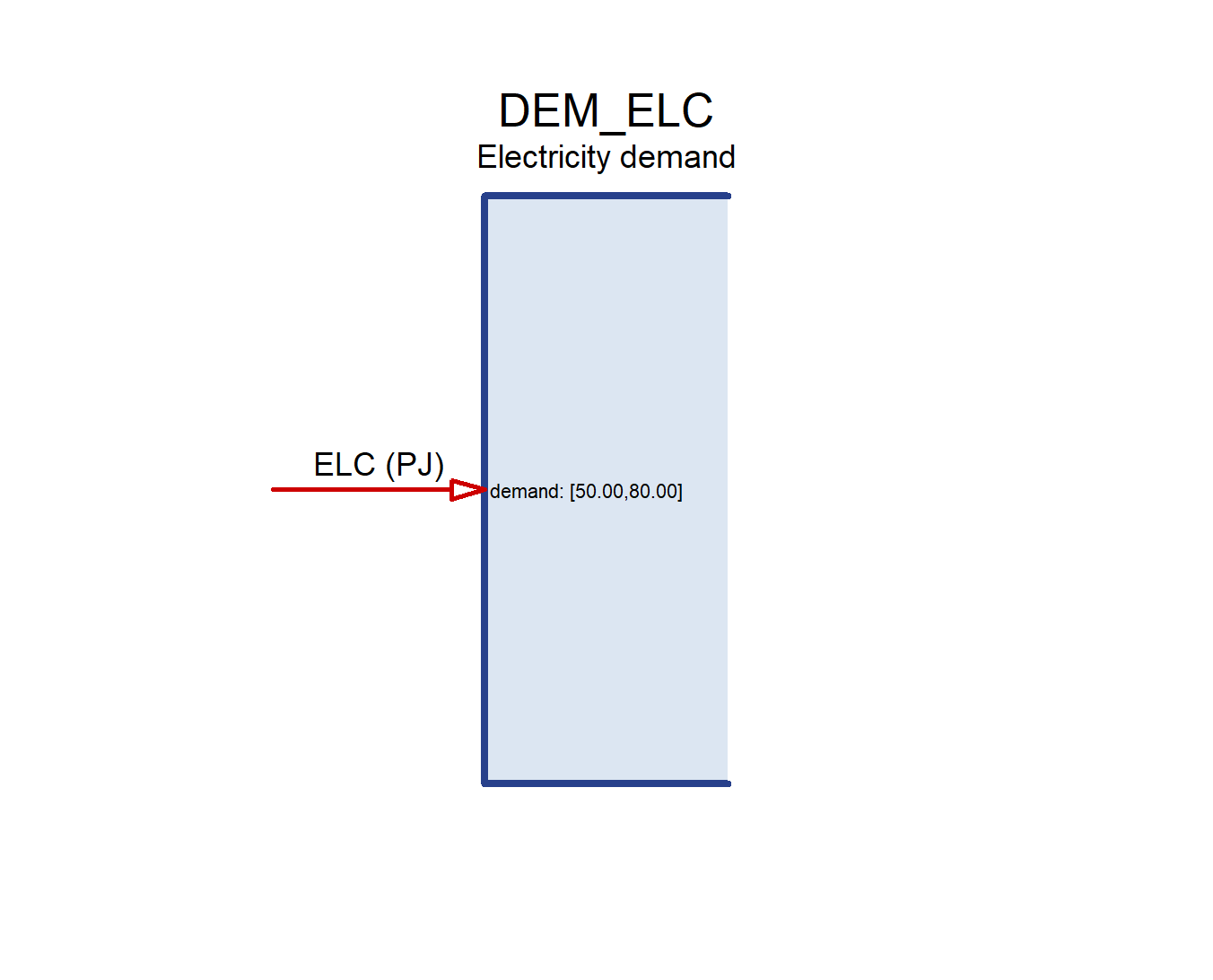
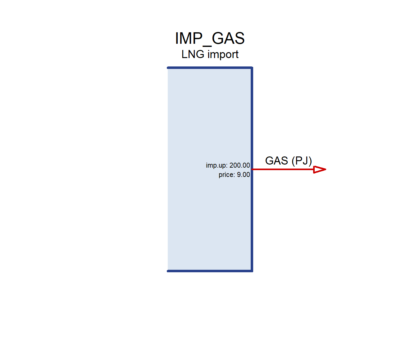
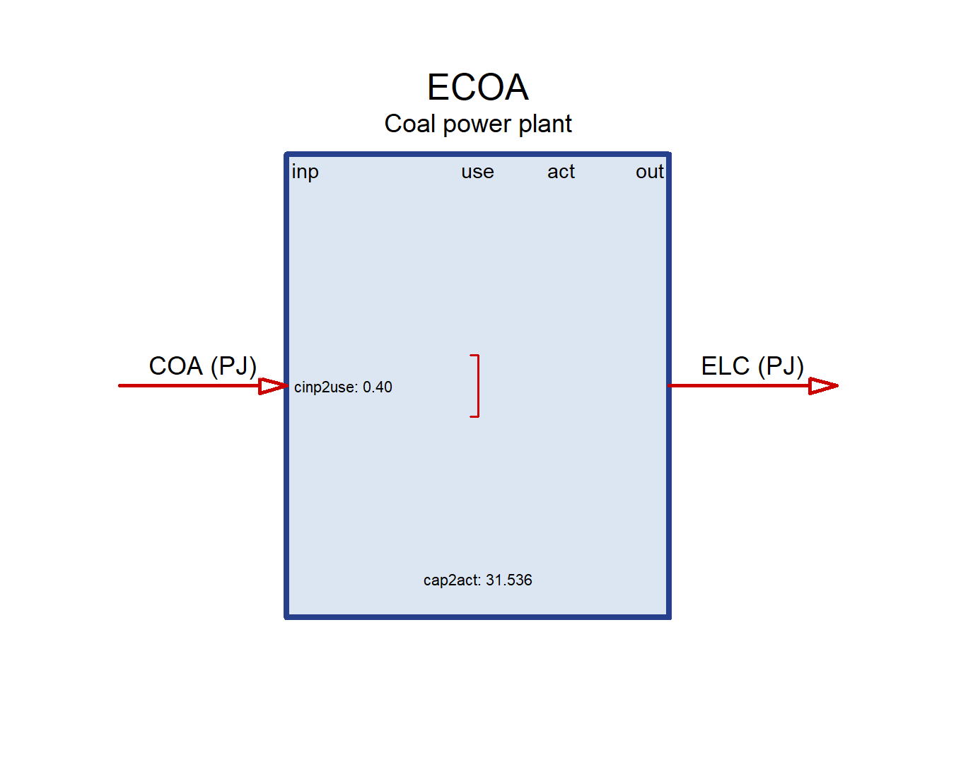
newConstraint(), newTax(), newSubsidy()Every process can be drawn: draw(obj) sketches its flows. We use it on every slide from here on.
Every constructor follows the same shape:
newTechnology(
name = "ECOA", # the set element -- UPPERCASE, no spaces
desc = "Coal power plant", # free text
input = list(comm = "COA"), # what it consumes
output = list(comm = "ELC"), # what it produces
ceff = data.frame(comm = "COA", cinp2use = 0.4), # parameters
region = character() # empty = every region
)name is the identifier the solver sees.data.frames, and may carry region, year, slice columns. Leave a column out and the value applies to all of them.newCommodity() — what flowsA commodity is a label with a unit. It has no diagram: it is the thing that travels along the arrows, not a box.
timeframe — the finest resolution at which this commodity balances. ANNUAL pools the year; HOUR forces hourly balancing.emis — emission factors travel with the fuel, so every technology that burns it inherits them (given combustion = 1 on the input).newSupply() — a domestic resourcenewDemand() — what must be servednewImport() — a flow from outsidenewTechnology() — the converter
Read the diagram left to right: inp → use → act → out.
Every technology has the same internal chain. Each arrow is a coefficient:
| Stage | Meaning | Coefficient |
|---|---|---|
inp |
commodity entering | — |
ginp |
grouped input, if declared | cinp2ginp |
use |
what the process actually consumes | cinp2use, ginp2use |
act |
activity — the capacity-linked variable | use2cact |
out |
commodity leaving | cact2cout |
cap2act converts capacity into annual activity (1 GW × 8760 h = 31.536 PJ).cinp2use = 0.40 alone describes a 40 % plant.Two fuels feeding one boiler. The group is the thing with an efficiency; the members compete for share within it.
ECOFIRE <- newTechnology(
name = "ECOFIRE",
input = list(comm = c("COA", "BIO"),
unit = c("PJ", "PJ"),
group = c("FUEL", "FUEL"),
combustion = c(1, 1)),
output = list(comm = "ELC", unit = "PJ"),
group = data.frame(group = "FUEL",
desc = "Boiler fuel", unit = "PJ"),
geff = data.frame(group = "FUEL",
ginp2use = 0.38),
ceff = data.frame(comm = c("COA", "BIO"),
cinp2ginp = c(1, 1),
share.up = c(1, 0.30)),
cap2act = 31.536, olife = 30L
)
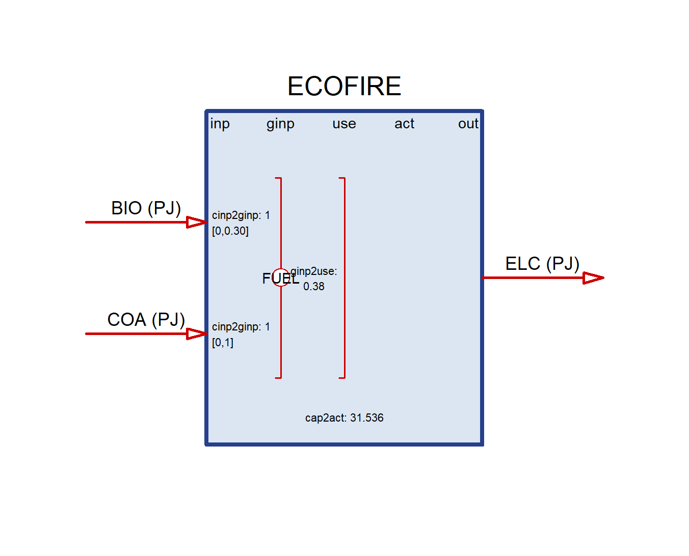
ginp column appears — it is absent for a single-fuel technology.FUEL is a node: both fuels flow into it, and it carries the efficiency (ginp2use: 0.38).[0, 0.30] next to BIO is the share bound: biomass may supply at most 30 % of the boiler’s fuel.[0, 1] next to COA: coal may supply all of it.. . .
Why group at all? Without a group each fuel would need its own efficiency and could not be constrained relative to the other. Shares are the point.
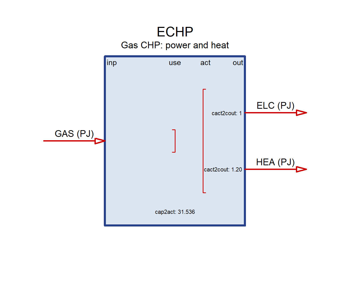
One activity, two products. cact2cout sets how much of each comes out per unit of activity.
ECHP <- newTechnology(
name = "ECHP",
desc = "Gas CHP: power and heat",
input = list(comm = "GAS", unit = "PJ",
combustion = 1),
output = list(comm = c("ELC", "HEA"),
unit = c("PJ", "PJ")),
ceff = data.frame(
comm = c("ELC", "HEA"),
cact2cout = c(1, 1.2) # heat/power ratio
),
cap2act = 31.536, olife = 25L
)Fixing both makes the ratio rigid; bound them instead for a flexible CHP.
Main commodities (red) are tied to capacity and activity. Auxiliary commodities (blue) are anything else the process consumes or emits — land, water, steel, labour, pollutants.
They are declared in aux, and linked in aeff by choosing which quantity they scale with:
| Coefficient | Scales with |
|---|---|
cinp2ainp, cinp2aout |
main commodity input |
cout2ainp, cout2aout |
main commodity output |
act2ainp, act2aout |
activity |
cap2ainp, cap2aout |
installed capacity |
ncap2ainp, ncap2aout |
new capacity (built this year) |
…ainp = the process consumes it, …aout = the process produces it.
ENUC <- newTechnology(
name = "ENUC",
desc = "Nuclear: land, water, steel",
input = list(comm = "NUC", unit = "PJ"),
output = list(comm = "ELC", unit = "PJ"),
aux = data.frame(
acomm = c("LAND", "WAT", "STEEL"),
unit = c("km2", "Mm3", "kt")),
aeff = data.frame(
acomm = c("LAND", "WAT", "STEEL"),
cap2ainp = c(0.5, NA, NA), # per GW held
act2ainp = c(NA, 0.02, NA), # per PJ made
ncap2ainp = c(NA, NA, 40) # per GW built
),
ceff = data.frame(comm = "NUC", cinp2use = 0.35),
cap2act = 31.536, olife = 50L
)
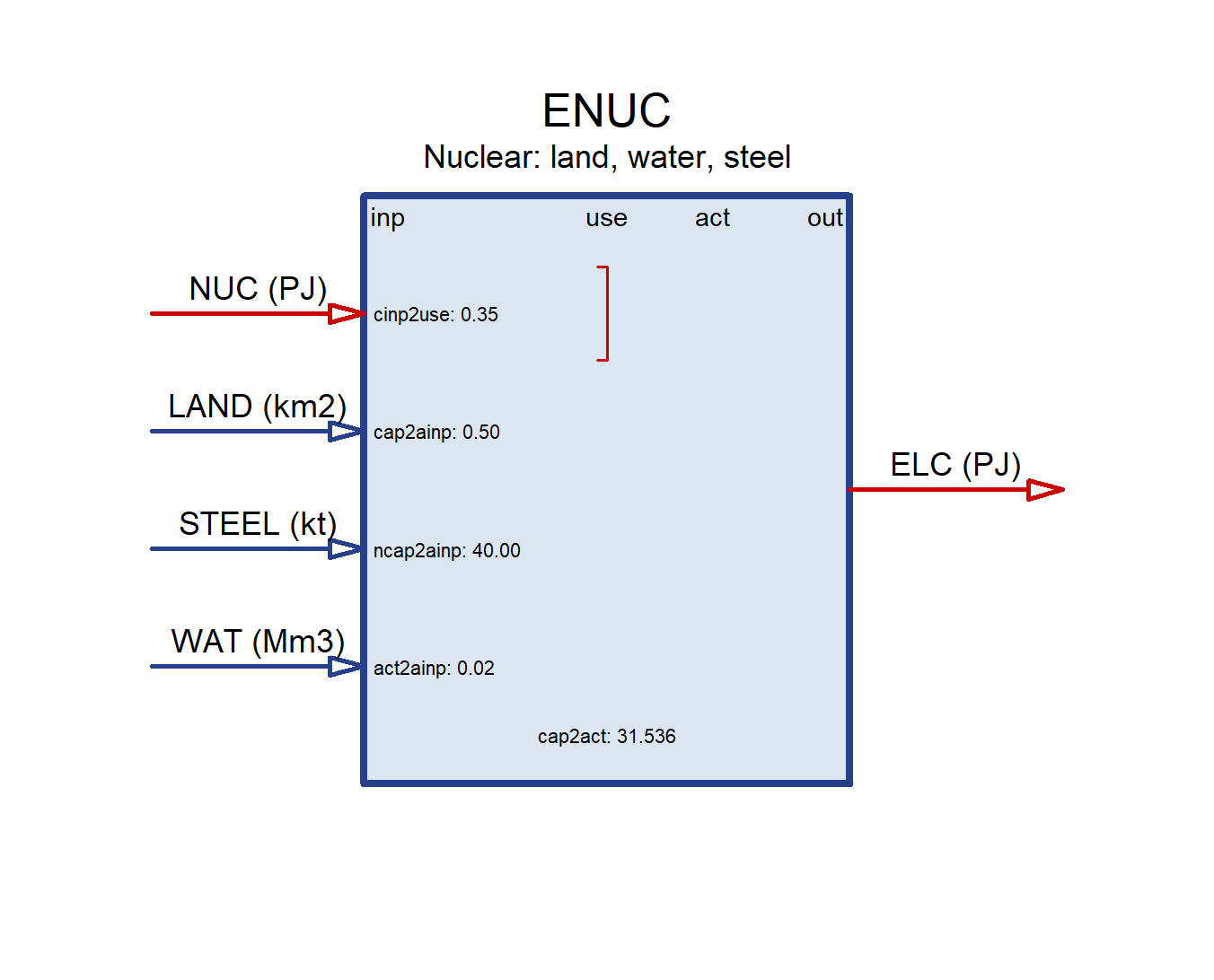
Three physically different things, and the diagram labels each one:
cap2ainp: 0.50 — land is occupied for as long as the plant stands, whether or not it runs.act2ainp: 0.02 — cooling water is drawn only when it generates.ncap2ainp: 40.00 — steel is consumed once, in the year the plant is built.. . .
Pick the wrong one and the model is quietly wrong: steel on cap2ainp would re-buy the whole plant every year.
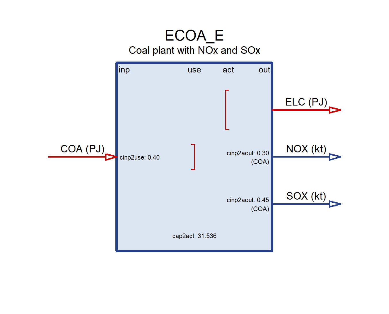
Pollutants that depend on the plant, not only the fuel, are auxiliary outputs scaled by fuel input:
ECOA_E <- newTechnology(
name = "ECOA_E",
desc = "Coal plant with NOx and SOx",
input = list(comm = "COA", unit = "PJ",
combustion = 1),
output = list(comm = "ELC", unit = "PJ"),
aux = data.frame(acomm = c("NOX", "SOX"),
unit = c("kt", "kt")),
aeff = data.frame(acomm = c("NOX", "SOX"),
comm = "COA",
cinp2aout = c(0.30, 0.45)),
ceff = data.frame(comm = "COA", cinp2use = 0.40),
cap2act = 31.536, olife = 30L
)Contrast with CO2, which sits on the commodity — every burner inherits it.
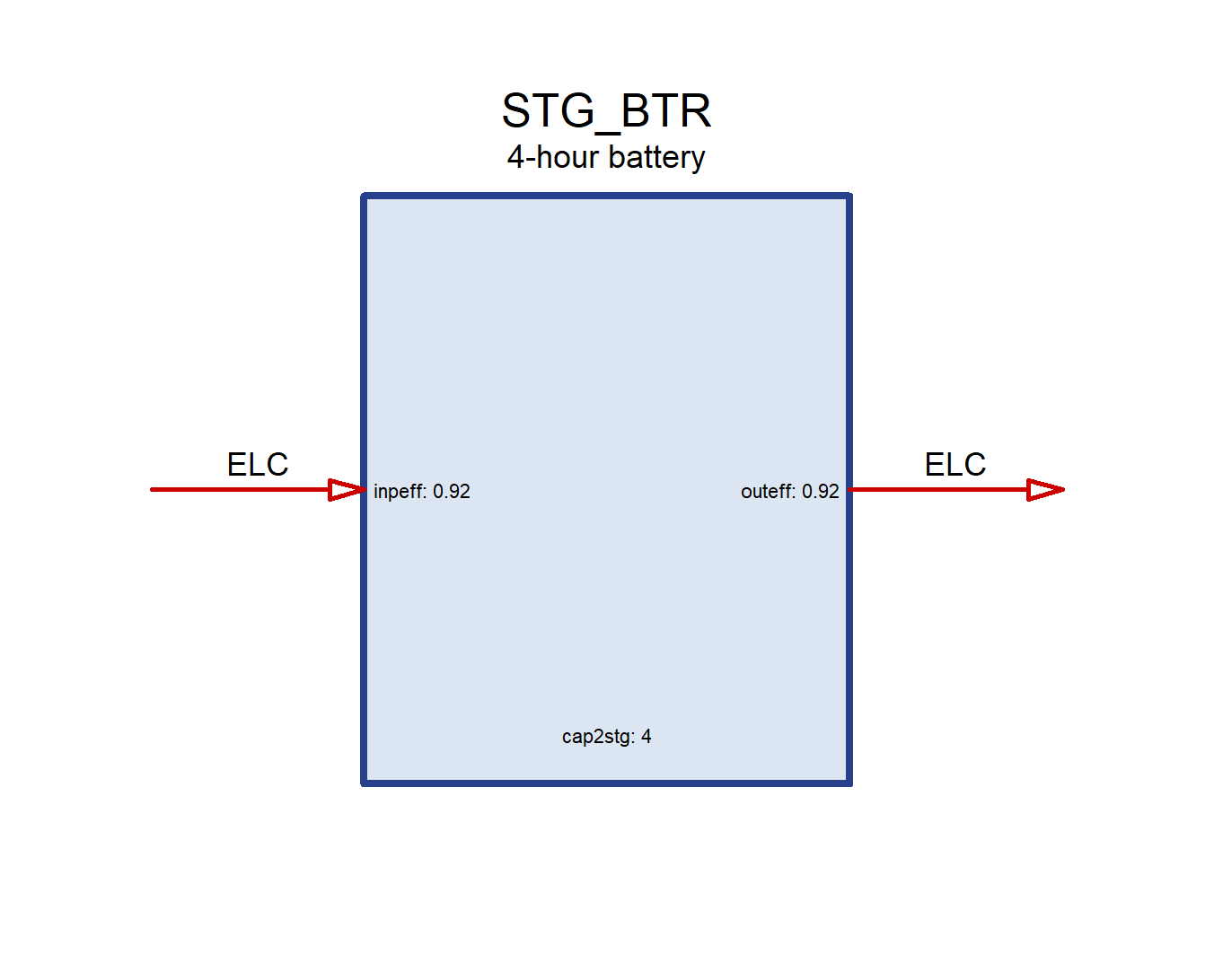
newStorage() — moving energy in timeseff — charge / discharge efficiency, and stgeff for standing losses.cap2stg — how many hours of storage one unit of capacity buys.
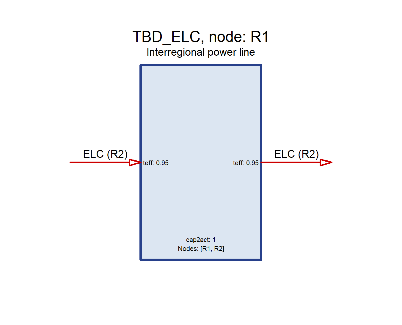
newTrade() — moving energy in spaceTBD_ELC <- newTrade(
name = "TBD_ELC",
desc = "Interregional power line",
commodity = "ELC",
routes = data.frame( # which links exist
src = c("R1", "R2"),
dst = c("R2", "R1")
),
trade = data.frame( # their parameters
src = c("R1", "R2"),
dst = c("R2", "R1"),
teff = 0.95 # line losses
),
invcost = list(invcost = 1500)
)Two slots, two jobs: routes declares the links, trade parameterises them. One is not derived from the other — a route with no parameters is unconstrained, and parameters for an undeclared route are ignored.
Trade is directional, so a bidirectional line is two rows in each. Note it has no region — the regions are src and dst.
newRepository() — the bagA repository is an ordered collection of objects. It has no behaviour of its own; it exists so a model can be assembled from named parts.
class: repository
objects: 8
add() / update() return a modified copy — nothing is mutated in place.newHorizon() and newModel()region — the model’s regions; objects with no region apply to all.horizon — milestone years. Periods grow, so the near term is resolved finely and the far term cheaply.interpolate_model() expands it over regions × years × slices; solve_scenario() solves it.| Function | Makes | Drawn? | Key arguments |
|---|---|---|---|
newCommodity() |
a flow | — | unit, timeframe, emis |
newSupply() |
a resource | ✔ | supply: cost, ava.up |
newDemand() |
an obligation | ✔ | demand |
newImport() / newExport() |
rest-of-world flow | ✔ | price, imp.up / exp.up |
newTechnology() |
a converter | ✔ | input, output, ceff, aeff, invcost |
newStorage() |
time shifting | ✔ | seff, cap2stg |
newTrade() |
space shifting | ✔ | routes, then trade: src, dst, teff |
newRepository() |
a bag of objects | — | name, ... |
newModel() |
the description | — | data, region, horizon |
When in doubt, draw() it. If the picture is not the system you meant, the model is not either.
A calendar declares the sub-annual structure every flow is balanced on. It is a set of nested timeframes, each split into slices carrying a share of the year.
ANNUAL SEASON DAYNITE slice share weight
<char> <char> <char> <char> <num> <num>
1: ANNUAL FA D FA_D 0.125 1
2: ANNUAL FA N FA_N 0.125 1
3: ANNUAL SP D SP_D 0.125 1
4: ANNUAL SP N SP_N 0.125 1
SEASON above DAYNITE gives 8 slices.newCalendar(name, timetable, year_fraction) turns a timetable into an object.Eight ship with the package — the fastest way to change a model’s time resolution is to swap one in.
[1] "season_dn" "d365"
[3] "utopia_annual" "utopia_seasons"
[5] "utopia_s4h24" "utopia_m12h24"
[7] "d365_h24" "d365_h24_subset_1day_per_month"
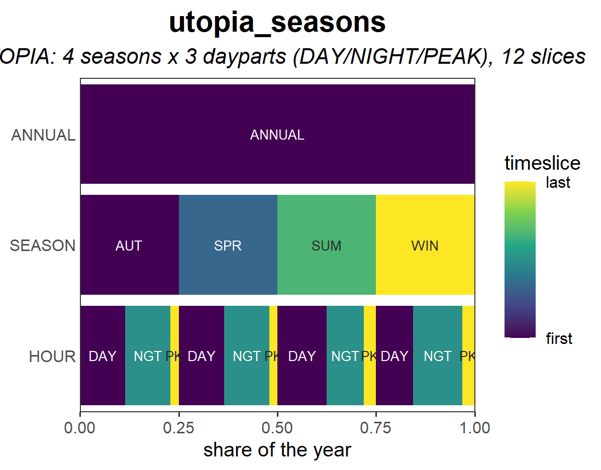
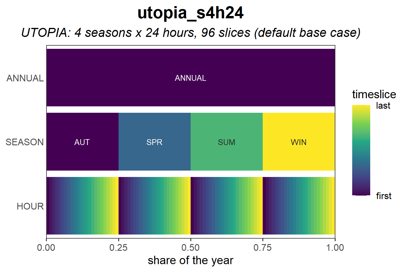

Each rectangle is one slice, sized by its share of the year. ANNUAL sits on top; finer timeframes stack below.
A sampled calendar keeps a representative subset of slices and declares what fraction of the year it covers:
slices year_fraction
sampled 288 0.0329
full 8760 1.0000
One day per month at hourly resolution — 288 slices instead of 8760, about 3.3 % of the year.
year_fraction is what keeps annual quantities honest when only part of the year is modelled.
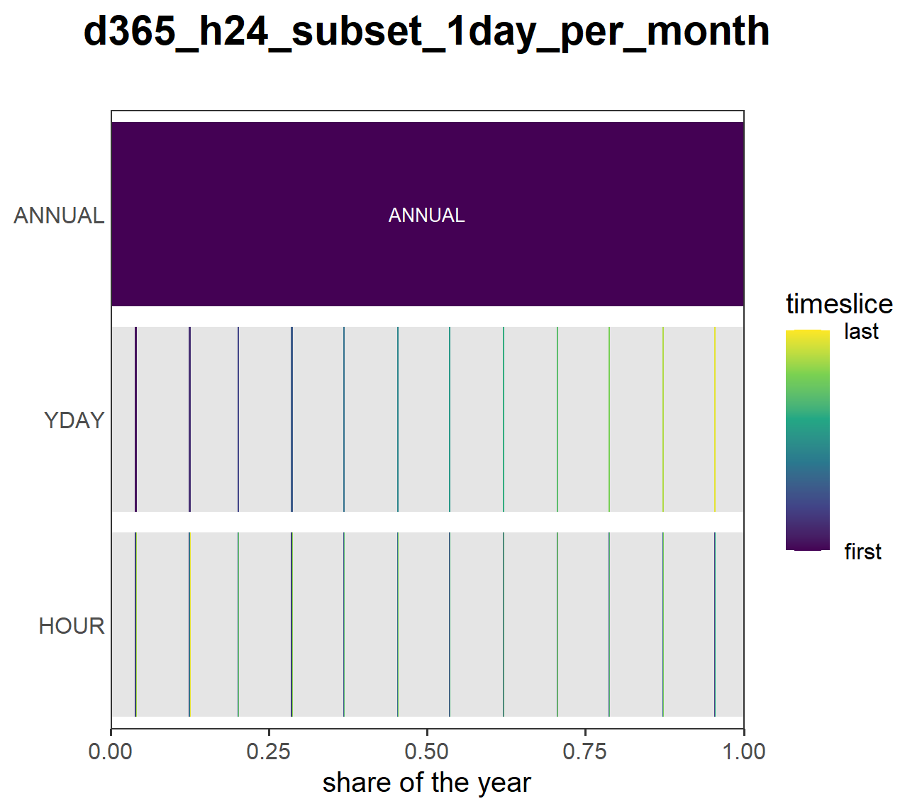
Passing reference = lays out the full structure and fills only the slices the sampled calendar declares.
Sampling reduces what is solved. Aggregation changes what you read back — getData() takes a timeframe argument:
timeframe = |
Returns |
|---|---|
"lowest" (default) |
flows summed up to the coarsest level, normally ANNUAL |
"highest" |
native resolution, as stored |
"all" |
every level, stacked |
"SEASON", "YDAY", … |
one named calendar level |
State variables (a storage level, say) are returned unchanged — summing a level over slices is meaningless, and the package knows the difference.
Roadmap planned
Nested timeframes and slice aggregation/disaggregation as a first-class operation move to the timescales package — the temporal companion to geoscales. Today energyRt’s calendar machinery is self-contained.
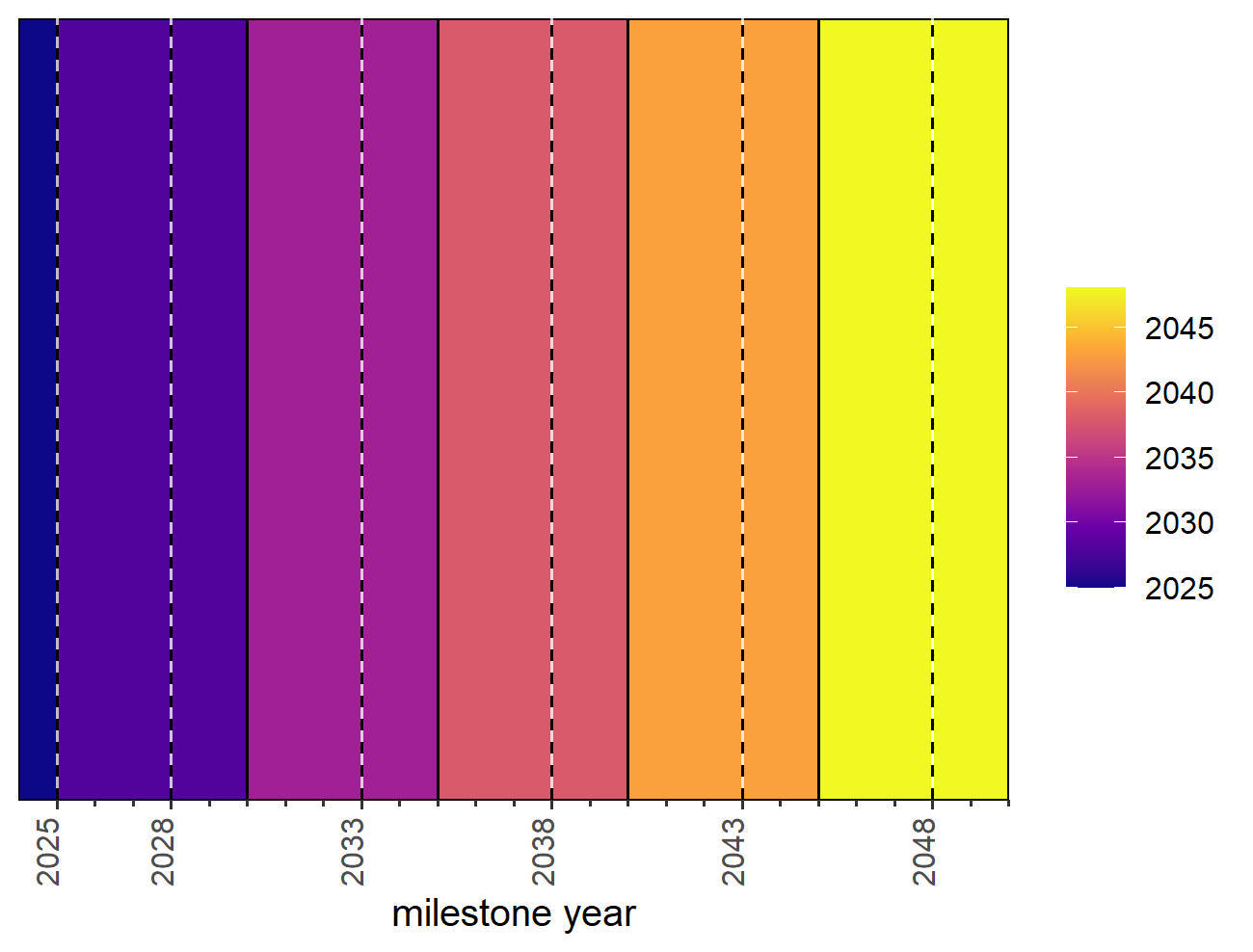
start mid end
<num> <num> <num>
1: 2025 2025 2025
2: 2026 2028 2030
3: 2031 2033 2035
4: 2036 2038 2040
5: 2041 2043 2045
6: 2046 2048 2050
period — the full span of years.intervals — either lengths (as here) or a data.frame with start, mid, end.force_BY_interval_to_1_year = TRUE).
The same intervals, three placements of the mid-year — the dashed line:
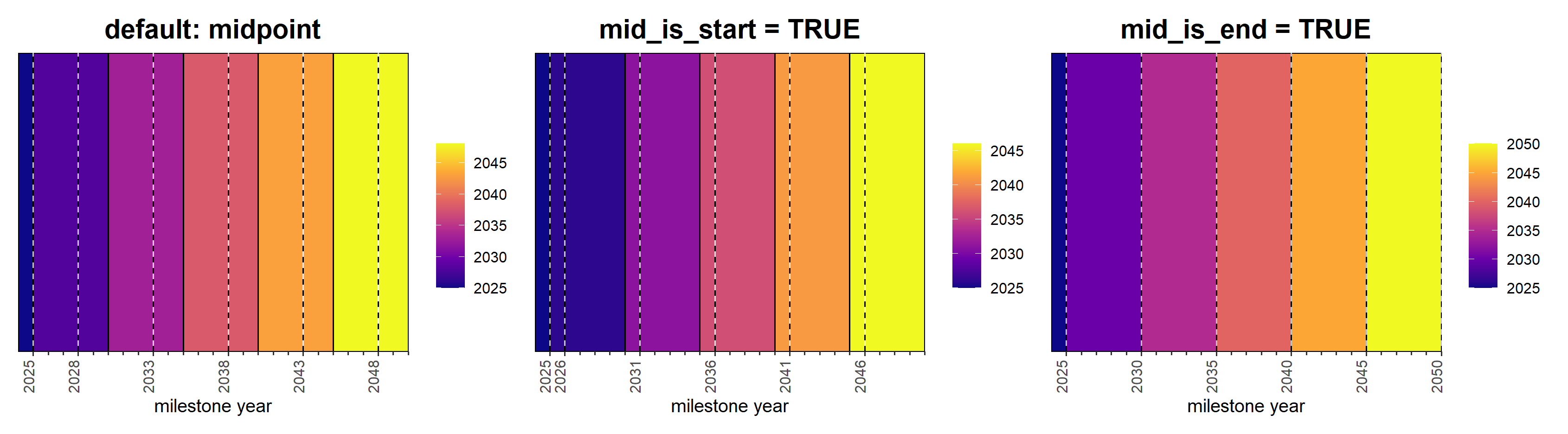
It matters because costs and demands are evaluated at the mid. mid_is_end puts the decision at the end of each period — the convention used in the models we build here. Choose once, and keep it consistent across scenarios you compare.
[1] "Y2020_2060_by_5" "Y2020_2060_by_10" "Y2020" "Y2030"
[5] "Y2040" "Y2050" "Y2060" "Y2070"
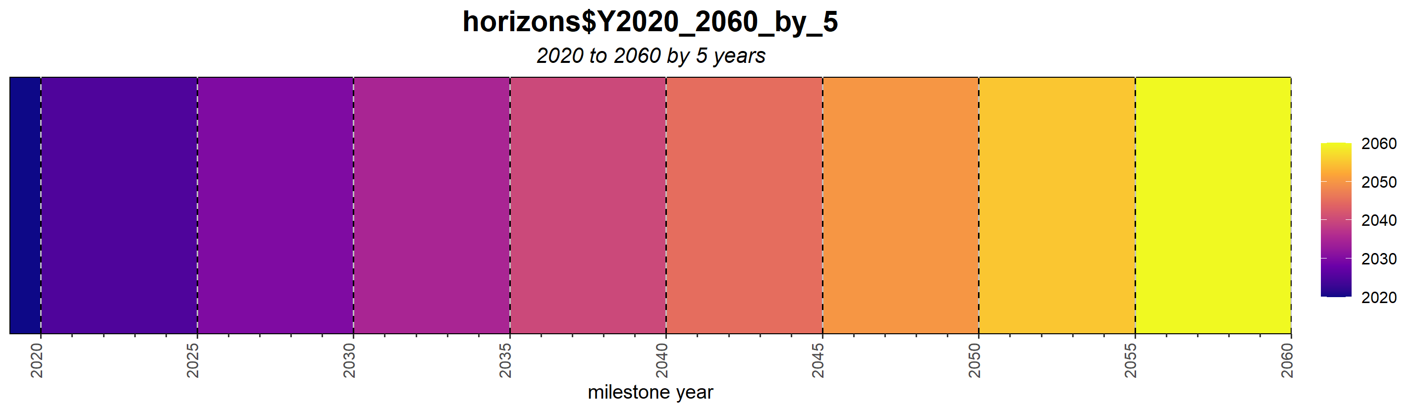
Single-year horizons (Y2030, Y2050, …) are useful for a fast structural check: build the model, solve one year, confirm it is feasible before paying for the full run.
There is no newRegion(). Regions are a flat character vector declared on the model:
region slot; leaving it empty means every region.trade is the exception — it has no region, only src and dst.get_region(obj) walks any object and reports the regions it refers to. It is deliberately schema-agnostic, so it keeps working as region information is added to classes that do not carry it yet.A geoscale (from the companion geoscales package) describes how regions nest into coarser levels, their weights, and optionally their geometry.
[1] "geoscales::Geoscale" "S7_object"
The one sentence to remember
A geoscale is used for plotting, reporting and subsetting only. Attaching one never changes the optimisation model. The extra members stay inert until some commodity names a coarser level.
setGeoscale() / getGeoscale() on a config, model or scenario.getData(..., geolevel = ) aggregates results up the hierarchy — "finest", "coarsest", "all", or a named level.plot_map() draws results on the geometry (needs sf).geolevel aggregation — summing a flow across regions would double-count it.| Slot | Decides |
|---|---|
name, desc |
identity |
limtype |
how the balance closes: LO (default, excess allowed), UP, FX |
timeframe |
where it balances in time — finest level in the model by default |
geolevel |
where it balances in space GLPK / GAMS only |
unit |
the commodity’s main unit |
emis |
emission factors carried by the fuel |
agg |
weights aggregating several commodities into this one |
misc |
free-form; never read by the model |
The commodity is deliberately lean: it is a label with balancing rules. All the engineering lives on the processes that consume and produce it.
In time — timeframe
Electricity must balance every hour; coal only has to balance over the year. Setting ANNUAL on a carrier that genuinely needs hourly matching is one of the easiest ways to build a model that is quietly too optimistic.
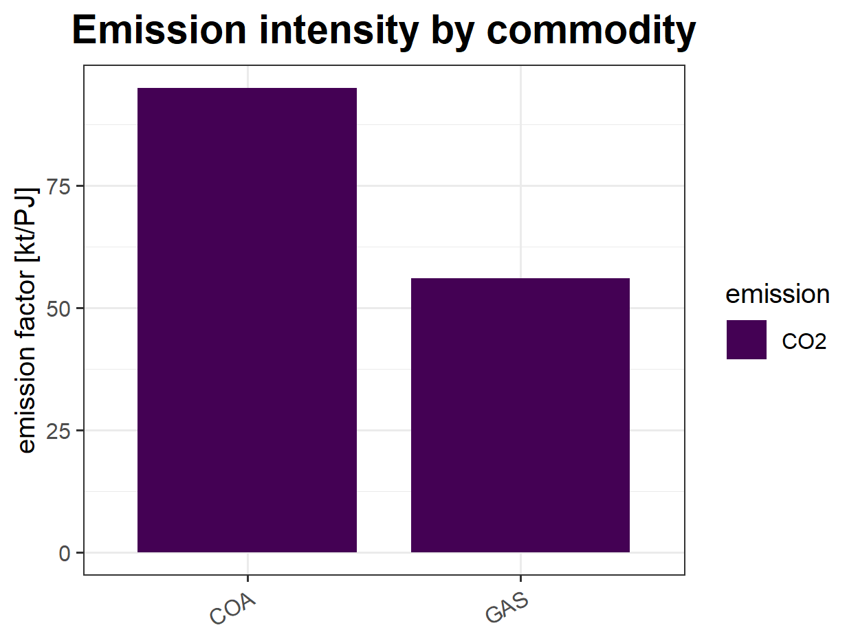
Emission factors ride on the fuel, so every technology burning it inherits them:
The factor only fires where the consuming technology declares combustion = 1 on that input.
There is no separate carbon-content slot — @emis is the single mechanism, and it generalises to any emitted species.
Roadmap planned
Physical properties — mass, volume, heating value — are not slots today, and @misc is the documented place to park them meanwhile. Adding them as first-class, unit-aware slots is a candidate for a future release.
A useful contrast, since both end up as “emissions”:
| Where it lives | Mechanism | Use when |
|---|---|---|
Commodity @emis |
factor per unit of fuel burned | CO2 — depends only on the fuel’s carbon |
Technology aeff cinp2aout |
auxiliary output scaled by input | NOx, SOx — depend on the burner, not just the fuel |
Two plants burning identical coal emit identical CO2 and quite different NOx. That is the whole distinction.
Real technologies are not one thing. A wind fleet has resource grades that differ in cost and yield, and build years that differ in efficiency and lifetime. energyRt expresses both on a single object:
| Dimension | Slot | Means |
|---|---|---|
| vintage | @vintage |
when it was built — investment window and operational life |
| cluster | @cluster |
which grade or variant it is — resource quality, siting class |
@vintage replaces the older start / end / olife slots: one row per (vintage, region, cluster) giving that variant’s window and life. A single row with vintage = NA is an ordinary un-vintaged technology.
The short form is usually enough — start and end default to the vintage year, so naming the years defines properly windowed vintages:
EWINVC <- newTechnology(
name = "EWINVC",
desc = "Wind: two resource grades, two vintages",
input = list(comm = "WIN"),
output = list(comm = "ELC"),
ceff = data.frame(comm = "WIN", cinp2use = 1),
cluster = data.frame(cluster = c("best", "mid"),
desc = c("High wind sites", "Medium wind sites"),
order = 1:2),
vintage = data.frame(vintage = c("2025", "2040"), olife = 25L),
invcost = data.frame(cluster = c("best", "best", "mid", "mid"),
vintage = c("2025", "2040", "2025", "2040"),
invcost = c(1400, 1150, 1600, 1300)),
cap2act = 31.536
)Nothing new was learned. Parameters vary by variant by gaining one more selector column — exactly like region or year. 2 × 2 = 4 cells, one object.
draw() reads the whole gridAsk for one cell and you get it, with the other vintages behind it as ghosts:
The faded stack is the vintage marginal through the selected cell — the cells sharing its cluster. Earlier vintages sit down-left, later ones up-right, so the depth of the stack is the technology’s history.
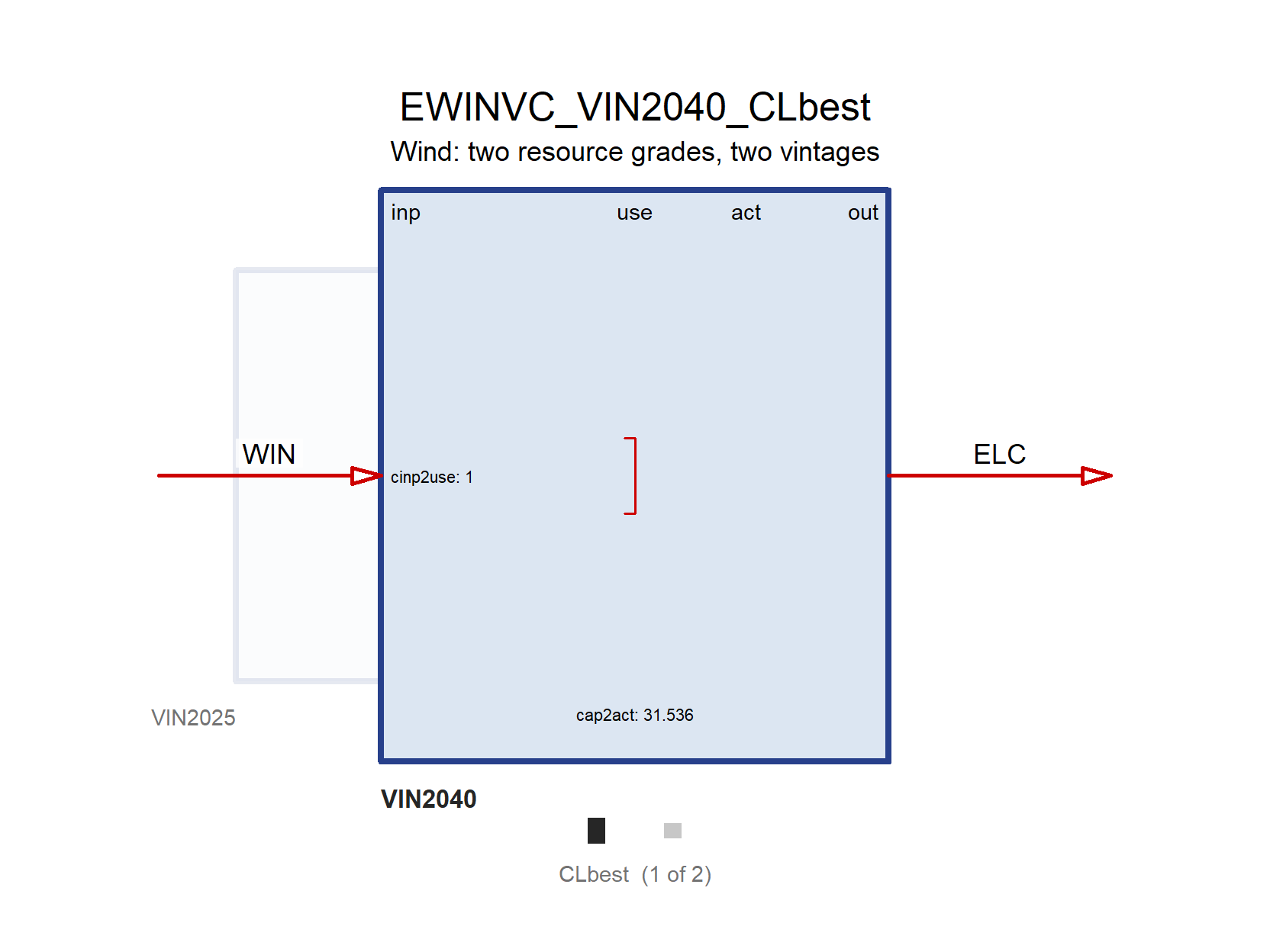
cluster_style changes how the sibling grades are rendered around the selected cell.
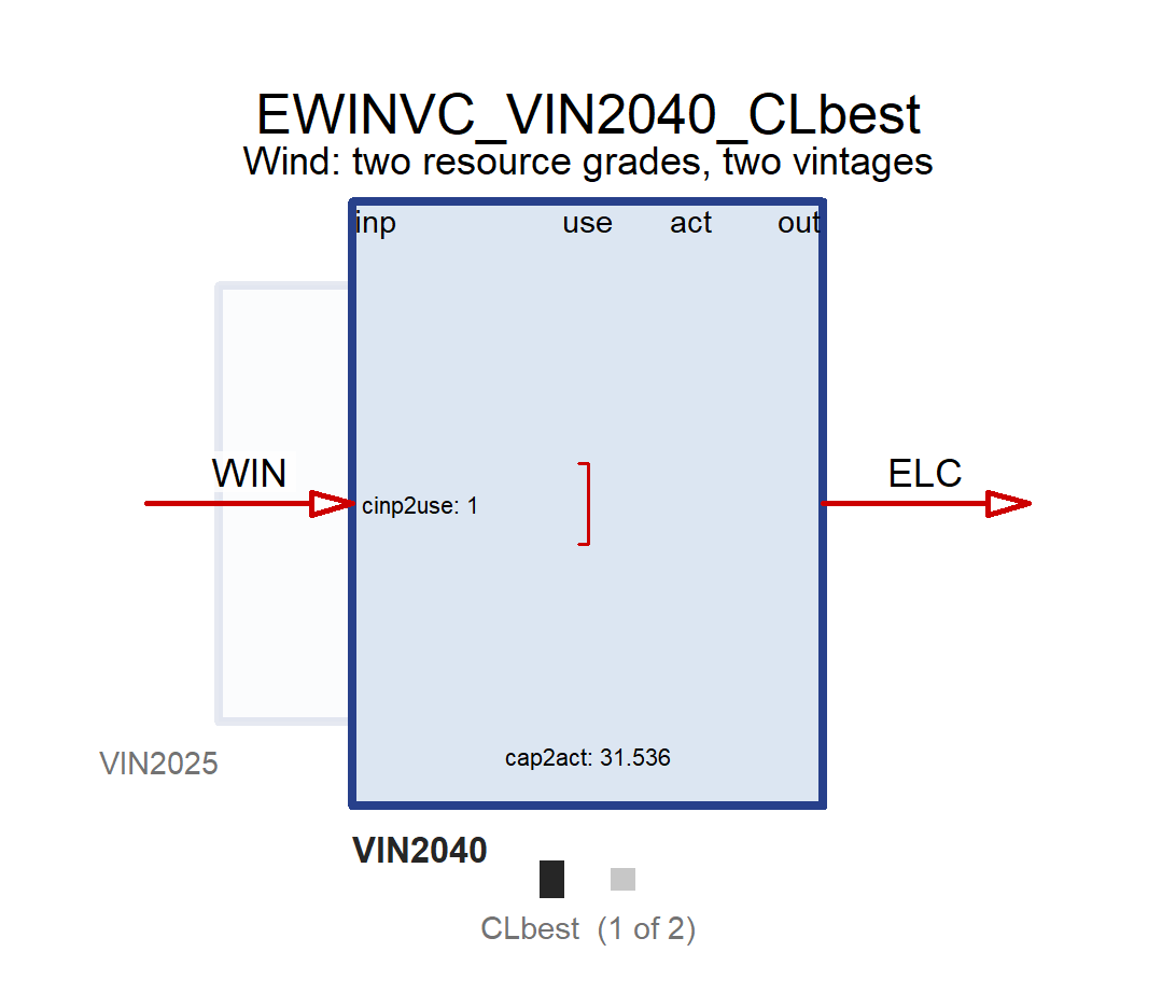
"rail" (default)
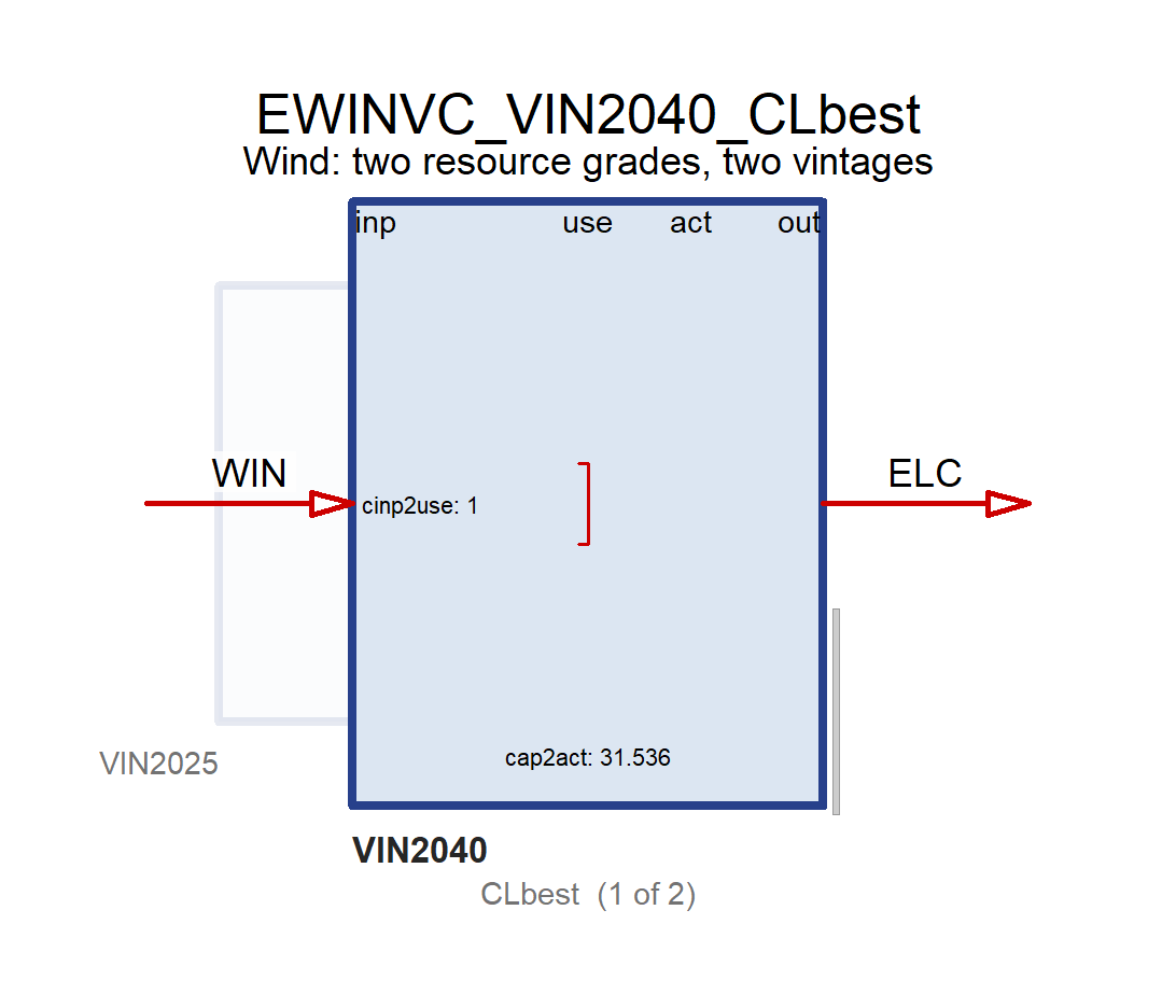
"deck"
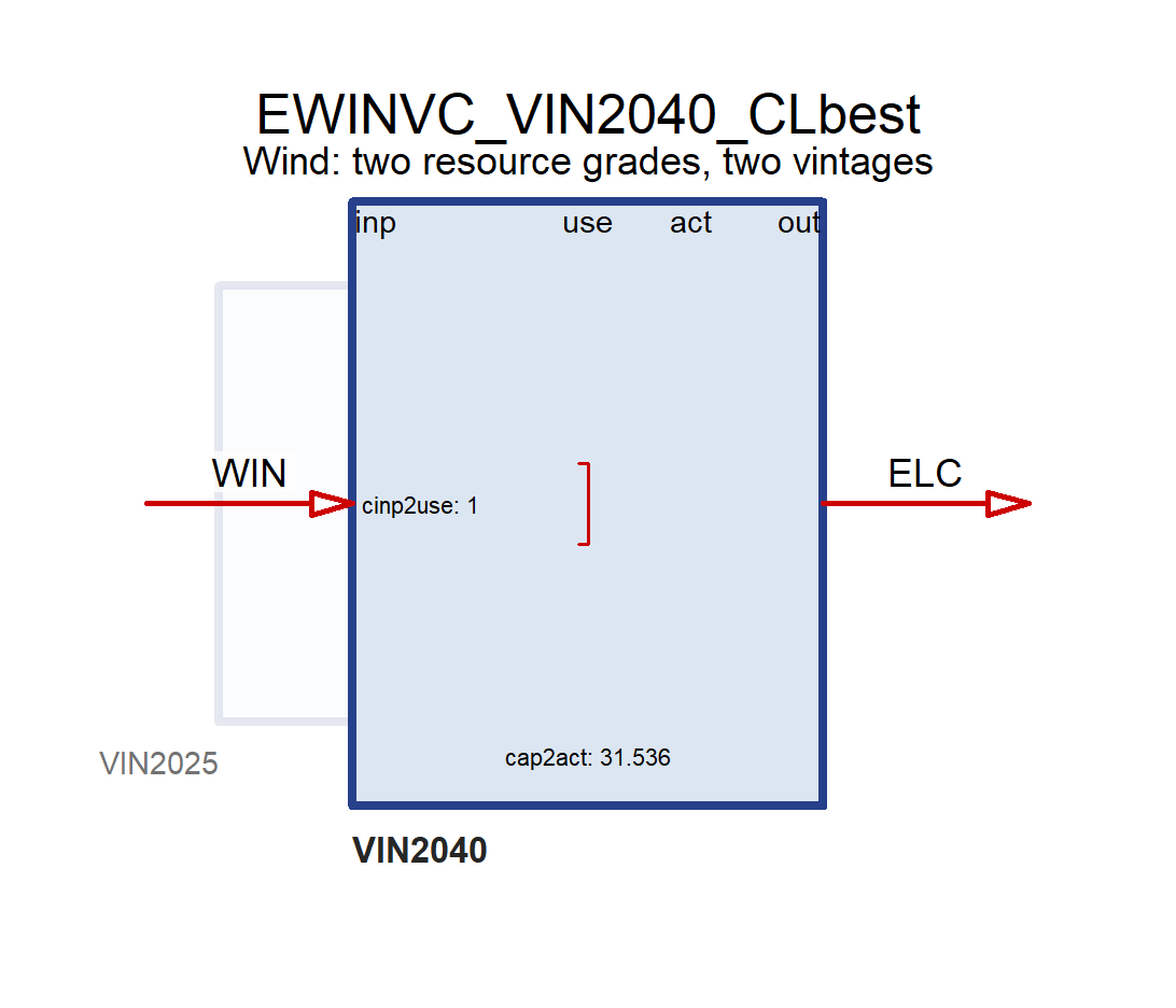
"none"
Cosmetic, not semantic — pick whichever makes the point on your slide.
Pass "all" to facet a dimension instead of selecting from it:
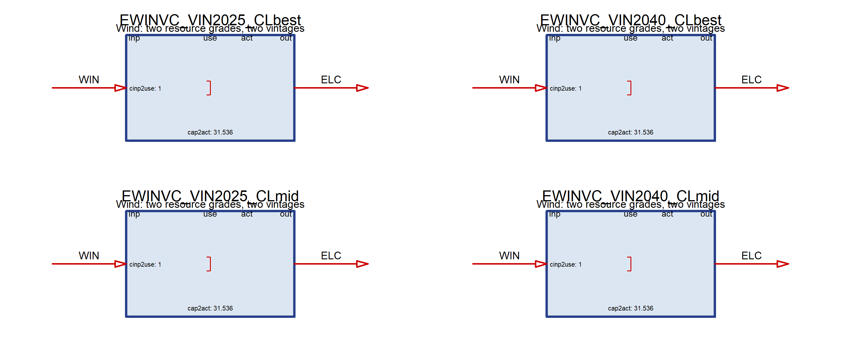
max_facets = 24L guards the obvious accident — a 4-vintage × 11-region technology asked to draw everything.
Variants are replicated into ordinary technologies before interpolation — the solver never sees the vintage/cluster idea, only more technologies.
Names gain a suffix from .variant_prefix, defaulting to _VIN and _CL: EWINVC becomes EWINVC_CLbest_VIN2025, EWINVC_CLmid_VIN2040, and so on.
design() — the object, back as codeUseful when an object came from a dataset or a colleague and you want to see what it actually says:
Returns (and can write to a file) the newTechnology() call that recreates it.
Note it renders the modern vintage table even when the object was built with the older olife = argument — a quick way to migrate old code.
technology only — no design() method for other classes yet.
ECOA <- newTechnology(
name = "ECOA",
desc = "Coal power plant",
input = data.frame(
comm = "COA",
unit = "PJ",
combustion = 1
),
output = data.frame(
comm = "ELC",
unit = "PJ"
),
ceff = data.frame(
comm = "COA",
cinp2use = 0.4
),
fixom = data.frame(
fixom = 55
),
invcost = data.frame(
invcost = 2000
),
vintage = data.frame(
olife = 30L
),
cap2act = 31.536
)interpolate_model() doesThe model object is a description. Interpolation compiles it into a solver-ready scenario:
Only step 3 is interpolation in the literal sense. Regions and slices are handled by expanding NA wildcards — an omitted region column means all regions, and it is expanded, not interpolated.
You supply anchor years; the pipeline fills the rest:
getData() returns both views — the given rows, and the interpolated series:
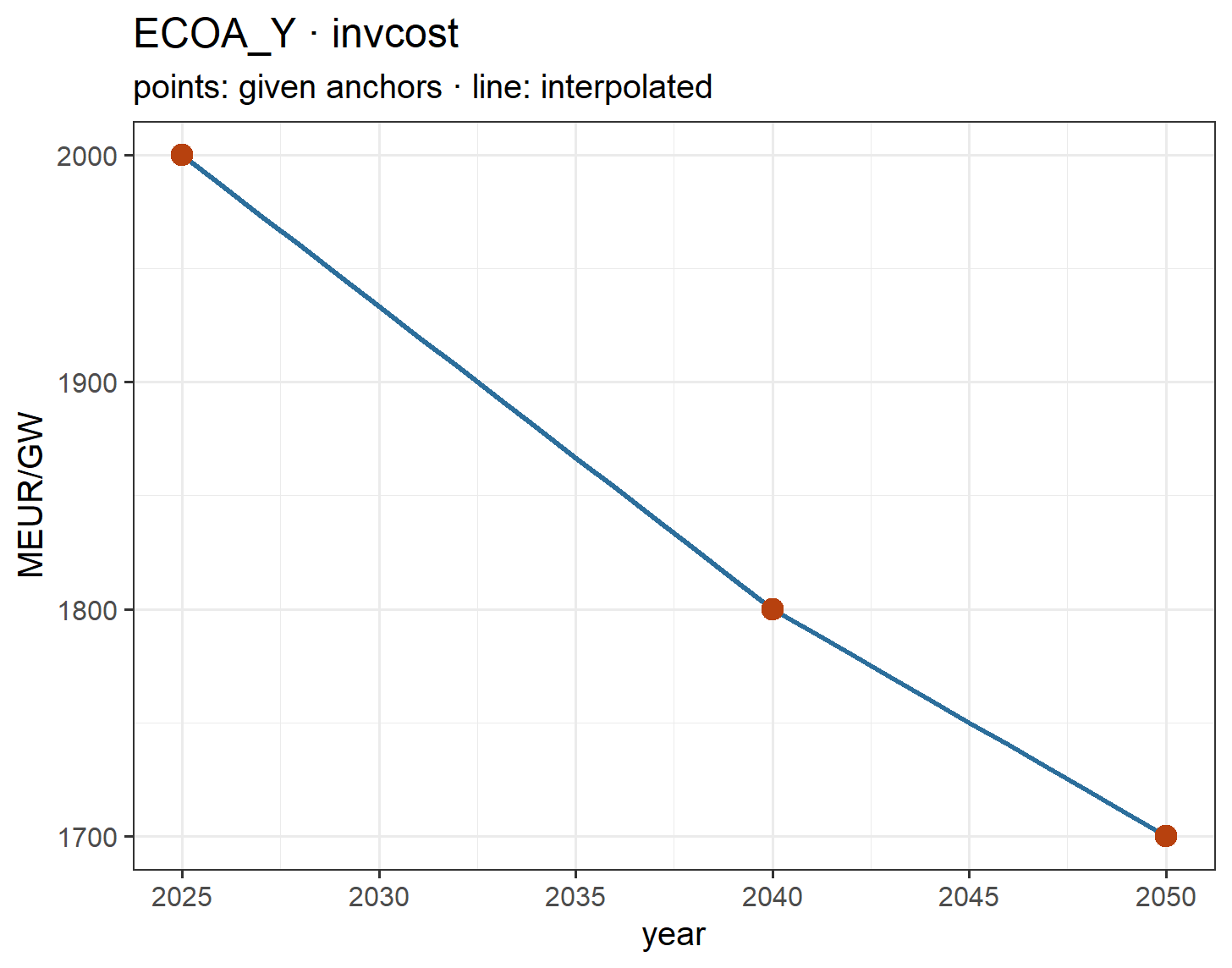
Each parameter carries a rule, stored as a composite of three tokens:
| Token | Alias | Applies |
|---|---|---|
back |
bwd |
before the first anchor — backward fill |
inter |
mid |
between anchors — linear |
forth |
fwd |
after the last anchor — forward fill |
The default nearly everywhere is back.inter.forth: constant outside the anchors, linear between them. That is why a single value with no year column becomes a flat line across the whole horizon.
Rules live in the config@interpolation table. To change them, build a modified config (or settings) and pass the object — there is no scalar interpolate_model(interpolation = ...) argument yet planned.
interpolate_model() accepts energyRt objects in ... and folds them into the model before the pipeline runs. That single mechanism is the whole scenario API:
| Pass an object of class | It replaces / adds |
|---|---|
calendar |
the scenario’s time structure |
horizon |
the milestone years |
config / settings |
the whole settings block |
repository |
added to the model |
technology, commodity, constraint, tax, … |
bundled into a scenario-specific repository |
Anything unrecognised is warned about, not silently ignored.
solve_scenario() / solve_mod() split their ...: run-control arguments stay, everything else is routed straight to interpolation.
The scenario folder name records what was swapped — {scenario}_{model}_{calendar}_{horizon} — computed from the final settings, so a substituted calendar shows up in the path:
COARSE_UTOPIA_utopia-seasons_base/
Not yet planned
Swapping regions, and named scalar overrides such as interpolate_model(mod, "S", discount = 0.07). Both are TODOs in the pipeline; for now, pass a full config/settings object.
model_size: BASE
parameters : 128 value, 233 maps, 13 sets
param rows : 5,902
estimate : ~16,111 variables, ~16,832 constraints (from gating maps)
top parameters by rows:
pTechCinp2use 1,536
pWeather 1,004
pSliceWeight 404
pSliceAgg 400
pDemand 384
model_size() counts parameter rows and estimates variables and constraints from the gating maps — enough to decide whether a run is worth starting.
| Operation | What it does | Lossless? |
|---|---|---|
| prune | drops rows whose value equals the parameter’s default | yes — an absent tuple reads back as the default |
| fold | replaces a whole column with NA wildcards where the value does not vary across the entire allowed membership |
yes — reversible with unfold_* |
| trim | drops rows that no equation-domain map indexes, i.e. data the model never reads | yes |
| densify | the opposite — materialises default rows, because GAMS has no parameter default and reads an absent tuple as 0 |
n/a |
GLPK / JuMP / Pyomo only — folding writes an artificial set member (ANYREGION, ANYSLICE, …) into the model source, and the substitution is not GAMS-ready yet.
Keep the same time structure, solve a representative subset of its slices — here every fourth hour of each season, and year_fraction records what is covered:
| scenario | calendar | slices | param_rows | variables |
|---|---|---|---|---|
| BASE | utopia_s4h24 | 96 | 5,902 | 16,111 |
| SAMPLED | utopia_s4h24_sampled | 24 | 1,614 | 4,231 |
A factor of roughly 4× in rows and variables, from one substituted object. Reduce the model before reaching for storage tricks.
Two different things, and only one of them exists today:
| What it does | Status | |
|---|---|---|
| Sampling | solve a subset of the calendar’s slices; year_fraction scales annual quantities |
works — substitute a sampled calendar |
| Aggregation | roll a fine calendar’s data up onto a coarser one — reweighting profiles, load curves, availability | in development |
Passing a structurally different, coarser calendar will build a smaller model, but the fine-resolution data is not aggregated onto it — that machinery is still being written, and lands with the timescales package. Until then, sampling is the supported way to shrink the time dimension of an existing model.
Aggregation on the results side already works: getData(timeframe = ) (Part 2).
Tip
Whichever route you take, compare_interp_settings() and compare_solve_settings() rebuild the same model across a grid of fold/sparse/prune settings and check the objective is invariant — the check worth running before trusting a reduction.
ondisk = TRUE writes each parameter to a modInp/ folder instead of holding it in @data.save_scenario() stores data-frame slots as parquet (zstd by default) and empties the in-memory slots; isInMemory() tells you which state an object is in.Two honest caveats
ondisk reduces peak memory during the build only — everything is materialised back into RAM before the solver files are written.
And getData() collects eagerly: the Arrow dataset is opened lazily, but filtering happens in R afterwards. There is no predicate push-down, so this is not larger-than-memory querying.
Everything above operates on parameter rows. Removing the variables and equations those rows would have gated is a different job — an equation-graph cascade: mark empty-domain variables, untrim the ones still referenced, drop the rest.
That cascade lives in the sibling multimod package (trim_model(), mark_empty_variables(), untrim_required_elements()), and energyRt does not call it yet. A partial removal on the energyRt side would leave dangling variable references in the equations that read them — which is precisely why it is not attempted here.
Integration with multimod is in progress and is the route by which this arrives.
getData() — one accessor, many sourcesKey arguments: timeframe and geolevel (aggregation, Parts 2–3), merge, process, parameters, variables, drop.zeros, asTibble.
The named list form is how many scenarios are compared — there is no need for a registry to hold them.
getMix() is the tidy extractor behind the scenario plot. Given a named list it row-binds with a scenario column, so any ggplot2 comparison is a facet_wrap(~ scenario) away.
autoplot() itself takes a single scenario — build multi-scenario charts from getMix().
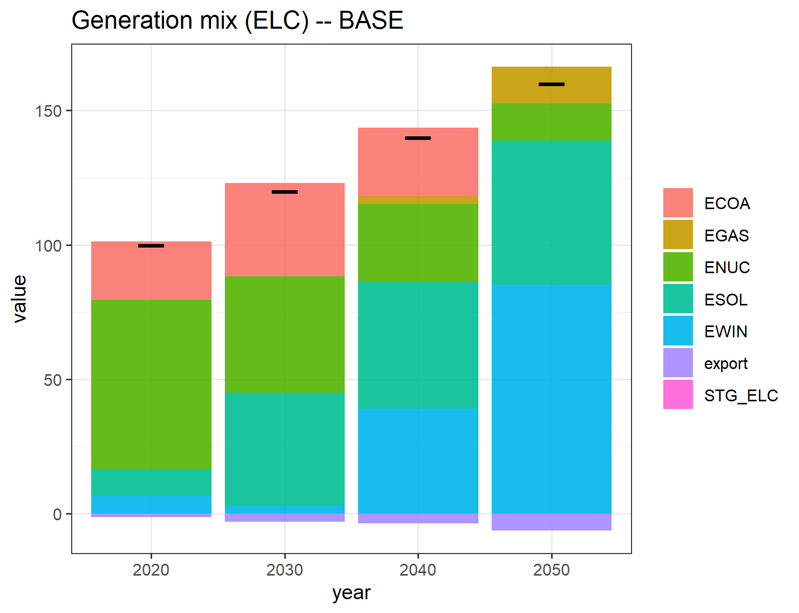
report() works on a technology, repository, model or solved scenario.html, pdf, tex — it downgrades to HTML with a warning if no LaTeX engine is found..Rmd to template =. The built-ins live in inst/templates/ (report_generic, report_model, report_scenario, report_vehicle).energyRt writes one linear program over all milestone years and solves it once: full perfect foresight. Every backend template contains a single solve statement.
That is a modelling assumption, not an implementation detail — the model knows the whole future when it invests. It is the right default for a least-cost benchmark and the wrong one for studying myopic behaviour.
Under development planned
Myopic · myopic with a guide or target · isolated regional solves · geo-aggregated solves · free/no-trade solves.
Also listed alongside these: coarse-time solving, which needs the aggregation machinery described in Part 8 — in development.
Time-sampled solving is the one you can already do today, by substituting a sampled calendar (Parts 2, 7 and 8).
| Backend | Needs locally |
|---|---|
| GLPK / MathProg | glpsol (ships with Rtools) |
| Julia / JuMP | Julia + HiGHS |
| Python / Pyomo | Python + CBC/HiGHS |
| GAMS | GAMS + a license |
| NEOS | nothing — an email address |
The same model object solves on any of them.
26 presets ship with the package. NEOS submits the model as inlined text, so a CPLEX solve needs no local GAMS at all — subject to its academic/non-commercial terms and a ~16 MB job cap.
Cross-solving one scenario on two backends and comparing objectives is the strongest correctness check available.
| Method | Returns | Defined for |
|---|---|---|
draw() |
grid schematic | technology, storage, supply, demand, import, export, trade |
autoplot() |
ggplot | 19 classes — calendar, horizon, commodity, weather, trade, demand, the processes, levcost, scenario, model, repository |
plot() |
ggplot | 17 classes — a thin delegate to autoplot() |
getData() |
tidy data | scenarios (and lists of them), models, repositories, single objects |
getObject() |
the objects | repository, model, scenario — filtered by class, name, region, … |
report() |
html / pdf / tex | technology, repository, model, scenario |
design() |
R code | technology only |
summary() / show() |
console | model, scenario, repository only |
Two things worth knowing before you go looking: there is no draw() for a model or repository — draw() describes a process, and report(mod) is what describes a whole model. And a process autoplot() needs year-indexed data in the economics or capacity slots; with none it returns NULL and says so.
While building
draw(obj) — is this the system I meant?design(tech) — what does this object actually say?getObject(repo, class = "technology") — what is in here?autoplot(cal), autoplot(hor) — is the time structure right?After solving
autoplot(scen) — the mixesgetMix(list(...)) — compare scenarioslevcost(scen, name =) — why did it pick that?model_size(scen) — why is this so slow?report(scen) — everything, in one documentThe escape hatch that avoids forking the model code:
In many cases this can be done without writing constraints in the GAMS, Julia/JuMP, Python/Pyomo, or GLPK-MathProg languages.
Each left-hand-side term is a summand: a variable, a multiplier mult, and what to sum it for.sum over.
experimental — and user constraints currently compile to GAMS-dialect text; moving them to a language-neutral form so every backend renders from one definition is in progress.
| Want to | Use |
|---|---|
| add a relationship between variables | newConstraint() experimental |
| add a cost term to the objective | newCosts() experimental |
| change what a report shows | report(template = "/path/to/your.Rmd") |
| carry your own metadata on any object | the @misc slot — never read by the model |
| change solver behaviour | solver_options$..., or set_option() / en_config_write() |
| add a new mapping to the pipeline | the mapping registry — a contributor path: declare it in modInp.yml, write map_<Name>(), register it |
Not available yet: newVariable() planned. The variable catalogue is fixed; a runtime constructor paralleling newConstraint() is on the roadmap. (The variable class you can see is the results container, not a constructor.)
Structure
geoscales and nested time via timescales — today both are flat sets with aggregation only on the reporting sidenewVariable(), to match newConstraint()commodity (mass, volume, heating value)Scale and solving
Most of the packages around energyRt are pre-release. If a piece of this is on your critical path, say so — that is the most useful thing you can tell us.
new*(), one grammar throughoutgetData(), autoplot(), levcost(), report()When in doubt, draw() it — and when the model is slow, model_size() it.
energyRt · useR! Training