Energy colour scales for ggplot2

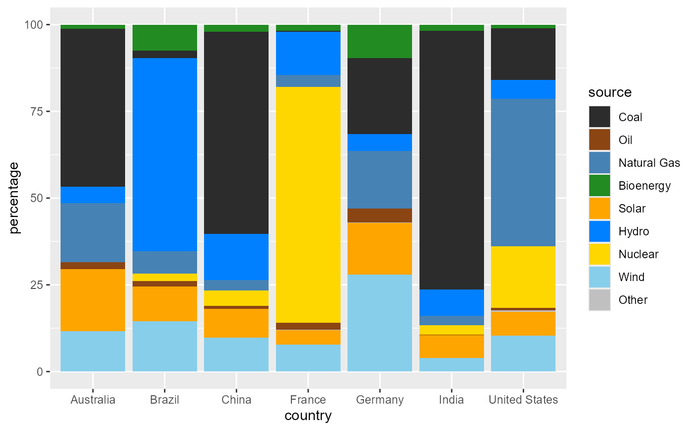
Colour the series of a plot from an energy palette. The discrete scale resolves whatever labels your data contains — "Coal", "nat gas", "COAL1" — through energypal_match(), so it works on real data without preprocessing. The _c and _b variants take a continuous palette and give a smooth gradient or binned steps.

Usage

scale_fill_energy(
  palette = NULL,
  file = NULL,
  order = NULL,
  direction = 1,
  label_style = c("asis", "id", "short", "long", "default"),
  unmapped_color = "#999999",
  gradient = FALSE,
  guide = "legend",
  ...
)

scale_colour_energy(
  palette = NULL,
  file = NULL,
  order = NULL,
  direction = 1,
  label_style = c("asis", "id", "short", "long", "default"),
  unmapped_color = "#999999",
  gradient = FALSE,
  guide = "legend",
  ...
)

scale_color_energy(
  palette = NULL,
  file = NULL,
  order = NULL,
  direction = 1,
  label_style = c("asis", "id", "short", "long", "default"),
  unmapped_color = "#999999",
  gradient = FALSE,
  guide = "legend",
  ...
)

scale_fill_energy_c(
  palette = "windatlas",
  file = NULL,
  direction = 1,
  na.value = "grey50",
  ...
)

scale_colour_energy_c(
  palette = "windatlas",
  file = NULL,
  direction = 1,
  na.value = "grey50",
  ...
)

scale_color_energy_c(
  palette = "windatlas",
  file = NULL,
  direction = 1,
  na.value = "grey50",
  ...
)

scale_fill_energy_b(
  palette = "windatlas",
  file = NULL,
  breaks = NULL,
  direction = 1,
  na.value = "grey50",
  ...
)

scale_colour_energy_b(
  palette = "windatlas",
  file = NULL,
  breaks = NULL,
  direction = 1,
  na.value = "grey50",
  ...
)

scale_color_energy_b(
  palette = "windatlas",
  file = NULL,
  breaks = NULL,
  direction = 1,
  na.value = "grey50",
  ...
)

Arguments

palette

Name of a built-in or registered palette. Defaults to the energypal.palette option, or "carriers" — except for _c() and _b(), which need a continuous palette and default to "windatlas".

file

Path to a palette file, taking precedence over palette.

order

Legend order. NULL keeps the data's own order; otherwise a declared ordering such as "carbon_intensity" or "merit_order", a computed one such as "alpha", or an explicit vector. See energypal_orders().

Presentation only — orderings arrange the legend and are not model inputs.

direction

1 (default) or -1 to reverse the order.

label_style

How to label the legend: "asis" (default) keeps the labels your data uses; "id" shows the canonical identifier; "short", "long" and "default" use the palette's display labels.

unmapped_color

Colour for labels the palette cannot resolve (default "#999999"), so they are visibly unmapped rather than silently wrong.

gradient

Logical; shade labels that resolve to the same carrier into distinct tones of it (default FALSE). See energypal_gradient().

guide, na.value, ...

Passed to the underlying ggplot2 scale.

breaks

For _b(), the bin boundaries. NULL (default) uses the palette's declared breaks.

Value

A ggplot2 scale, to be added to a plot with +.

Choosing a variant

scale_fill_energy()

discrete data: carriers, technologies, sectors.

scale_fill_energy_c()

continuous data with a smooth ramp.

scale_fill_energy_b()

continuous data in bins, using the palette's own break points unless you override them. This is how resource maps are conventionally drawn.

Passing a continuous palette to the discrete scale, or the reverse, is an error rather than a silent half-result.

See also

energypal() for the palette, energypal_colors() for the colours alone, energypal_orders() for the available orderings.

Examples

if (requireNamespace("ggplot2", quietly = TRUE)) {
  library(ggplot2)
  d <- subset(owid_energy_mix, year == max(owid_energy_mix$year))

  # the data says "Coal", "Natural Gas", "Oil" - no preprocessing needed
  ggplot(d, aes(country, percentage, fill = source)) +
    geom_col() +
    scale_fill_energy()

  # a published colour scheme
  ggplot(d, aes(country, percentage, fill = source)) +
    geom_col() +
    scale_fill_energy(palette = "ipcc")

  # order the stack by carbon intensity rather than alphabetically
  ggplot(d, aes(country, percentage, fill = source)) +
    geom_col() +
    scale_fill_energy(order = "carbon_intensity")
}