The palettes • energypal

library(energypal)
library(ggplot2)
library(dplyr)

Every palette is a YAML file under inst/extdata/palettes/, carrying its own colours, labels, aliases and provenance. This article previews all of them.

Nothing here is hard-coded: the sections below are generated from energypal_info(), so a palette added to the store appears without this file being edited.

What is installed

info <- energypal_info()

info |>
  select(name, title, type, n, unit) |>
  knitr::kable()

name	title	type	n	unit
carriers	Energy carriers	discrete	93	NA
eia	EIA Annual Energy Outlook (approximation)	discrete	12	NA
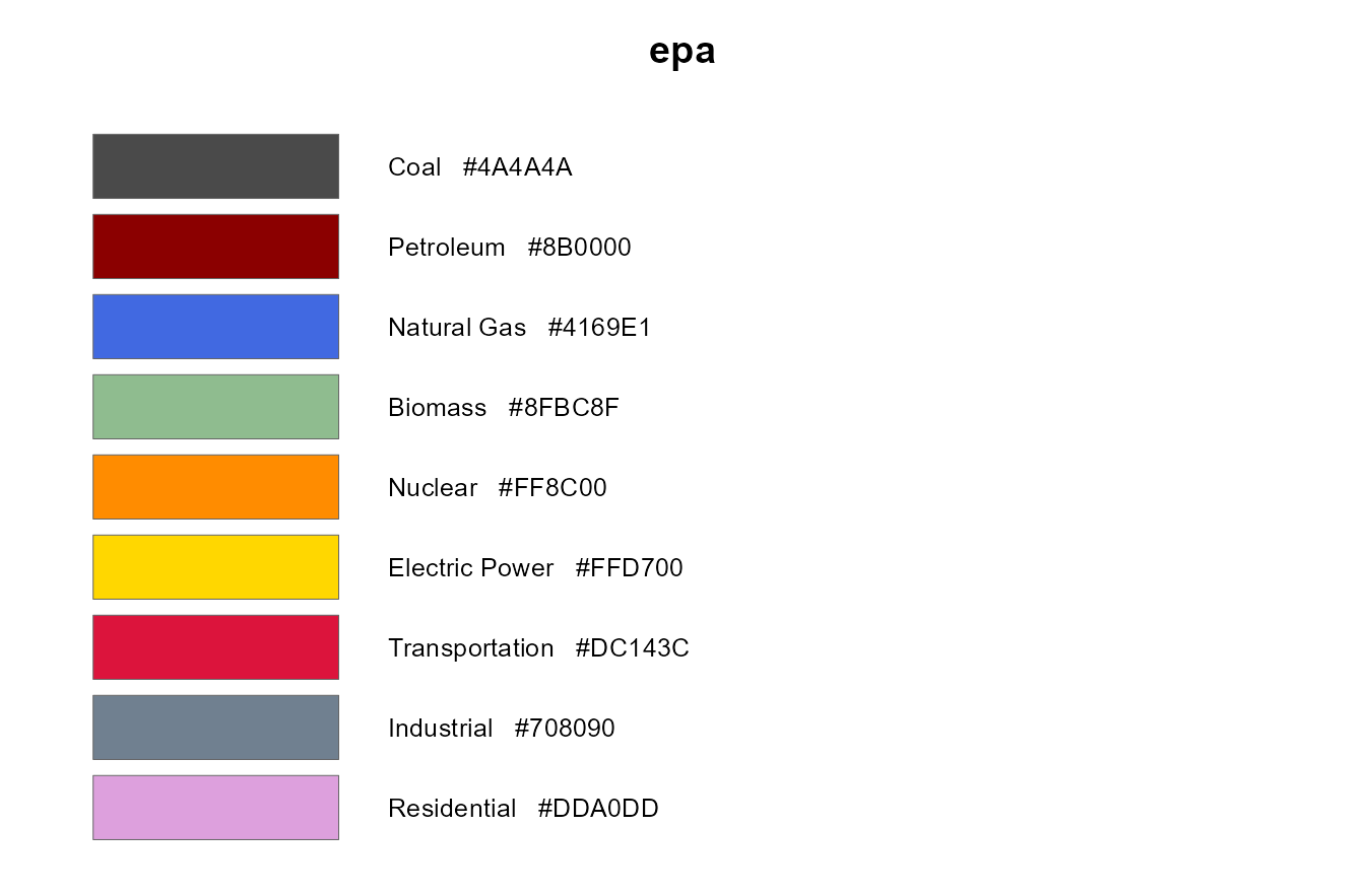
epa	EPA greenhouse gas inventory (approximation)	discrete	12	NA
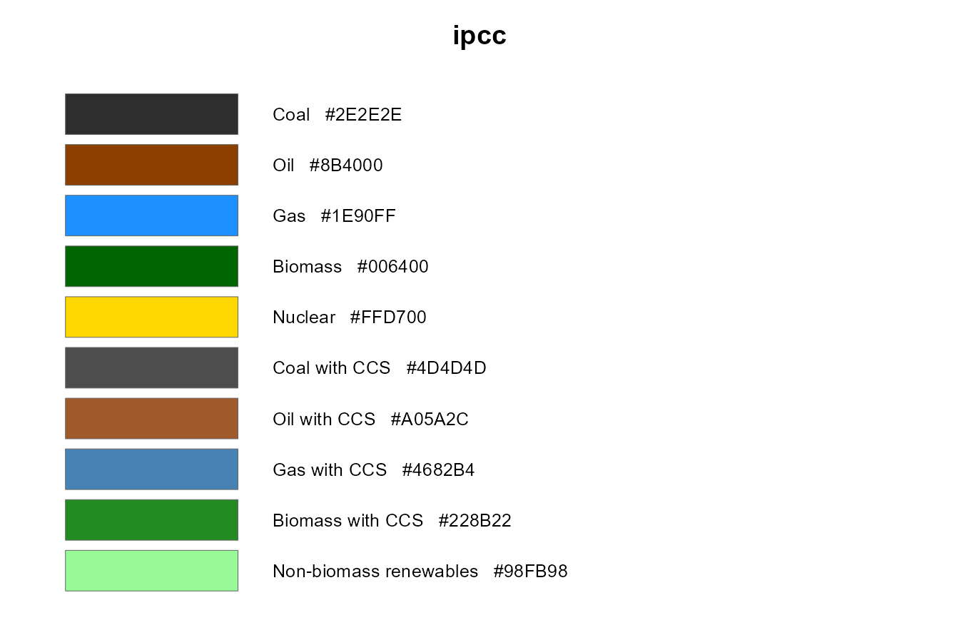
ipcc	IPCC AR6 WGIII energy supply (approximation)	discrete	11	NA
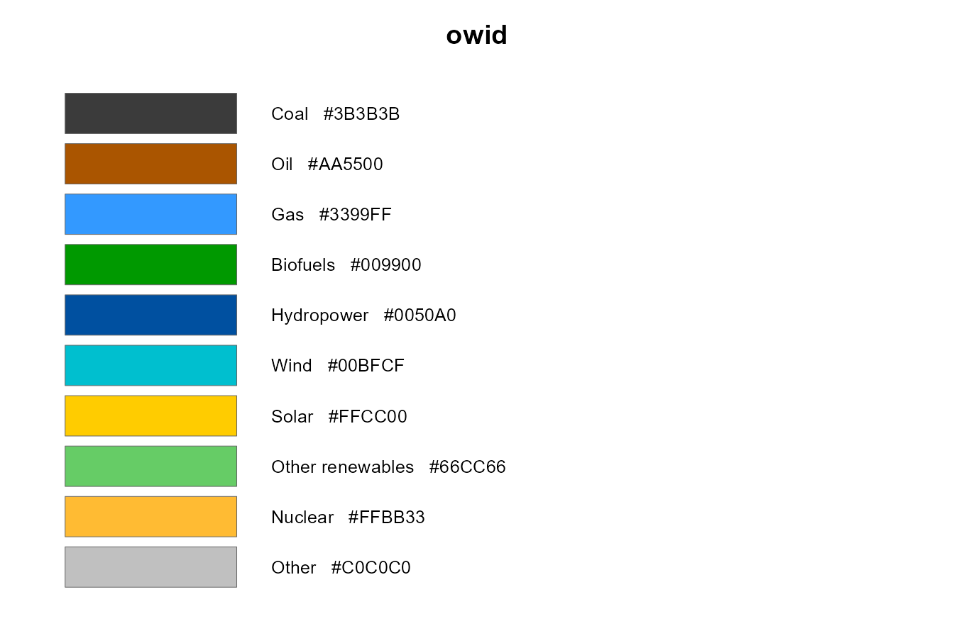
owid	Our World in Data energy mix (approximation)	discrete	12	NA
solaratlas_ghi	Global Solar Atlas GHI	continuous	28	kWh/m2/yr
solaratlas_pvout	Global Solar Atlas PV output	continuous	24	kWh/kWp
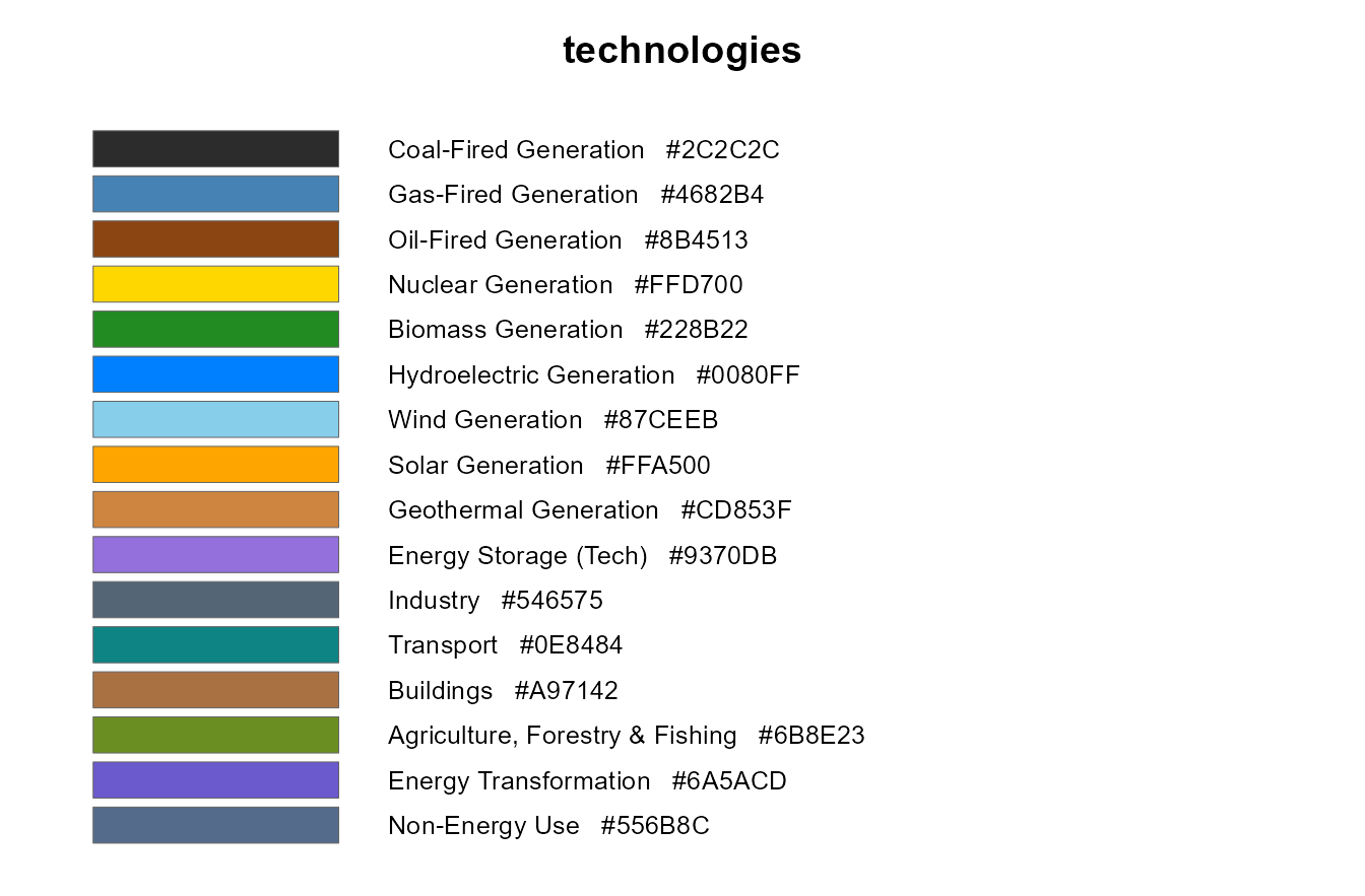
technologies	Energy technologies and sectors	discrete	80	NA
windatlas_speed	Global Wind Atlas mean wind speed (approximation)	continuous	31	m/s

The two kinds are handled differently throughout, so it is worth naming them once:

discrete <- info |> filter(type == "discrete") |> pull(name)
continuous <- info |> filter(type == "continuous") |> pull(name)

discrete
#> [1] "carriers"     "eia"          "epa"          "ipcc"         "owid"        
#> [6] "technologies"
continuous
#> [1] "solaratlas_ghi"   "solaratlas_pvout" "windatlas_speed"

All at a glance

Given several names, energypal_show() draws them as aligned rows — one per palette, one column per entry. Differences between published schemes are easier to see this way than in any table.

energypal_show(discrete)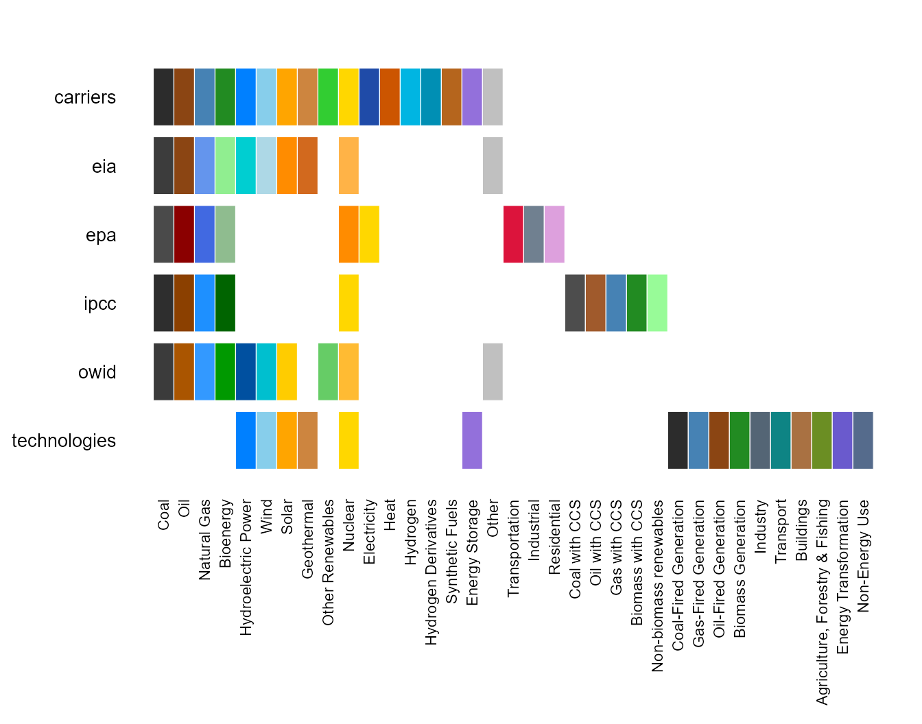

Entries that only some palettes define trail off to the right: IPCC’s CCS variants, EPA’s sector categories, the technologies taxonomy.

Continuous palettes have no entries to align on, so several of them are drawn stacked instead, each with its own range and unit:

energypal_show(continuous)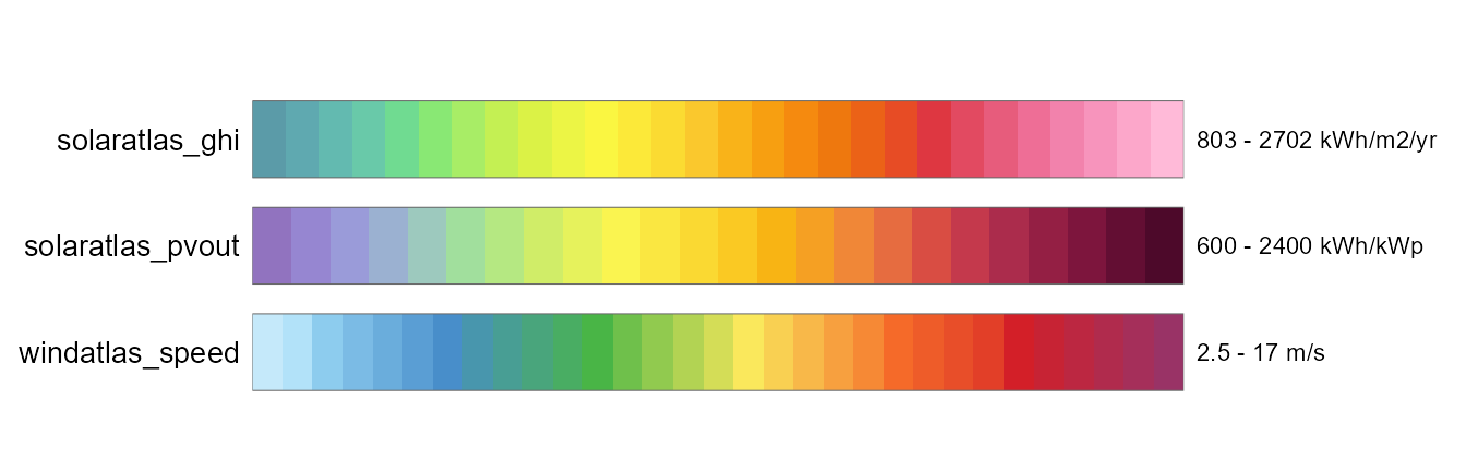

Discrete palettes

A palette shows only the colours its own source publishes. Report palettes extends: carriers, which gives them the taxonomy — names, labels, aliases, hierarchy, orderings — but not its colours. So a carrier a source is silent about comes back unmapped rather than quietly borrowing the default:

setdiff(names(energypal("carriers")), names(energypal("owid")))
#> [1] "Geothermal"          "Electricity"         "Heat"               
#> [4] "Hydrogen"            "HydrogenDerivatives" "SyntheticFuels"     
#> [7] "Storage"

# OWID publishes no geothermal series, and says so
energypal_match("Geothermal", palette = "owid", warn = FALSE)
#>     original    matched color      method candidates
#> 1 Geothermal Geothermal  <NA> unpublished       <NA>

# ...while the inherited alias vocabulary still resolves
energypal_colors("nat gas", palette = "owid", warn = FALSE)
#>   nat gas 
#> "#3399FF"

That is why these palettes are worth choosing between: each is its source’s own set, not the default with a few edits. Three earlier palettes (iea, fossil, renewable) were dropped for failing that test — iea differed from carriers in zero carrier-level entries, because carriers was seeded from it.

for (nm in discrete) {
  spec <- energypal_spec(nm)
  m <- spec$meta

  cat("\n### ", if (is.null(m$title)) nm else m$title, "  \n", sep = "")
  cat("`", nm, "`\n\n", sep = "")
  if (!is.null(m$source)) cat("**Source** ", m$source, "  \n", sep = "")
  if (!is.null(m$url))    cat("**URL** <", m$url, ">  \n", sep = "")
  if (!is.null(m$extends)) cat("**Extends** `", m$extends, "`  \n", sep = "")
  if (!is.null(m$license)) cat("\n> **Licence** ", m$license, "\n", sep = "")
  if (!is.null(m$attribution)) {
    cat("\n> **Attribution** ", m$attribution, "\n", sep = "")
  }
  cat("\n")

  energypal_show(nm, label_style = "default")
  cat("\n\n")
}

Energy carriers

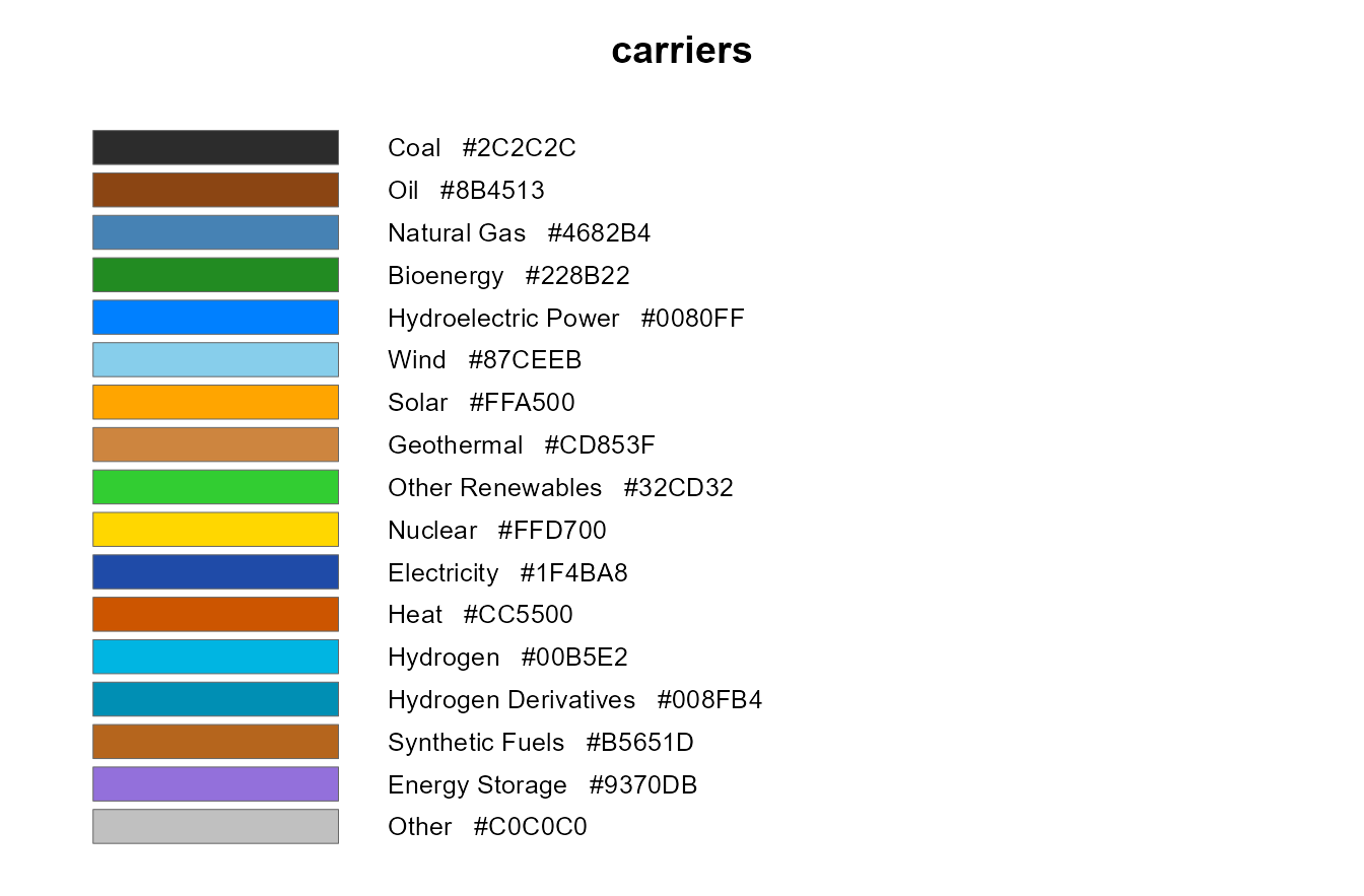
carriers

Source IPCC 2006 Guidelines, IEA World Energy Balances, EIA fuel categories
URL https://www.ipcc-nggip.iges.or.jp/public/2006gl/

Licence Colours are energypal’s own, following IEA World Energy Outlook conventions (dark grey coal, blue gas, orange solar, pale blue wind). They are not reproduced from any single published figure. The taxonomy follows the classifications cited per branch as _taxonomy_source; see dev/references/palette-licences.md

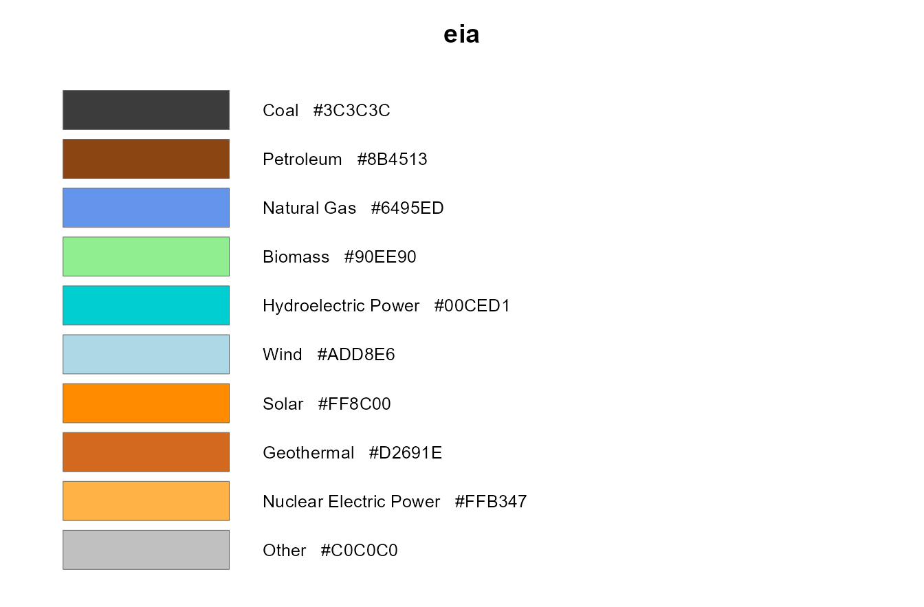
EIA Annual Energy Outlook (approximation)

eia

Source EIA Annual Energy Outlook 2023, Fig. ES-1 “Energy consumption by source”
URL https://www.eia.gov/outlooks/aeo/
Extends carriers

Licence Public domain. A work of the U.S. federal government, not subject to copyright protection in the United States (17 U.S.C. 105). Colours approximated from published figures; see dev/references/COLOR_REFERENCES.md

EPA greenhouse gas inventory (approximation)

epa

Source EPA Inventory of U.S. Greenhouse Gas Emissions and Sinks, Ch. 2 “Trends in Greenhouse Gas Emissions”
URL https://www.epa.gov/ghgemissions/inventory-us-greenhouse-gas-emissions-and-sinks-1990-2021
Extends carriers

Licence Public domain. A work of the U.S. federal government, not subject to copyright protection in the United States (17 U.S.C. 105). Colours approximated from published figures; see dev/references/COLOR_REFERENCES.md

IPCC AR6 WGIII energy supply (approximation)

ipcc

Source IPCC AR6 WGIII, Chapter 3, Fig. 3.8 “Energy Supply in Illustrative Pathways”
URL https://www.ipcc.ch/report/ar6/wg3/downloads/report/IPCC_AR6_WGIII_Chapter03.pdf
Extends carriers

Licence IPCC material may be reproduced with acknowledgement of the source. Colours approximated from a published figure, not an IPCC specification; see dev/references/report-palettes-survey.md

Attribution Colours after IPCC, 2022: Climate Change 2022 - Mitigation of Climate Change. Contribution of Working Group III to the Sixth Assessment Report of the Intergovernmental Panel on Climate Change, Chapter 3, Figure 3.8. Approximated from the published figure; not an IPCC colour specification.

Our World in Data energy mix (approximation)

owid

Source Our World in Data, “Energy Mix” interactive charts
URL https://ourworldindata.org/energy-mix
Extends carriers

Licence CC BY 4.0. Colours approximated from published figures; see dev/references/report-palettes-survey.md

Attribution Colours after Our World in Data, “Energy Mix” (https://ourworldindata.org/energy-mix), licensed CC BY 4.0. Approximated from published charts; not an official OWID specification.

Energy technologies and sectors

technologies

Source IEA Energy Technology Perspectives, IPCC 2006 Guidelines (Vol.2 Energy)
URL https://www.ipcc-nggip.iges.or.jp/public/2006gl/

Licence Colours are energypal’s own, derived from the carriers palette so that a technology and the carrier it consumes read as the same family. They are not reproduced from any published figure. The sectoral groupings follow IEA and IPCC conventions; see dev/references/palette-licences.md

Continuous palettes

Resource maps need a ramp rather than a set of categories. These palettes are an ordered list of stops and declare their own break points and unit, so a binned scale needs no configuration.

for (nm in continuous) {
  spec <- energypal_spec(nm)
  m <- spec$meta
  brk <- as.numeric(unlist(spec$breaks))

  cat("\n### ", if (is.null(m$title)) nm else m$title, "  \n", sep = "")
  cat("`", nm, "` — family `", m$family, "`, measure `", m$measure,
      "`, unit `", m$unit, "`  \n", sep = "")
  cat(length(energypal(nm)), " stops, ", length(brk), " breaks from ",
      min(brk), " to ", max(brk), "  \n", sep = "")
  if (!is.null(m$source)) cat("**Source** ", m$source, "  \n", sep = "")
  if (!is.null(m$license)) cat("\n> **Licence** ", m$license, "\n", sep = "")
  if (!is.null(m$attribution)) {
    cat("\n> **Attribution** ", m$attribution, "\n", sep = "")
  }
  cat("\n")

  energypal_show(nm)
  cat("\n\n")
}

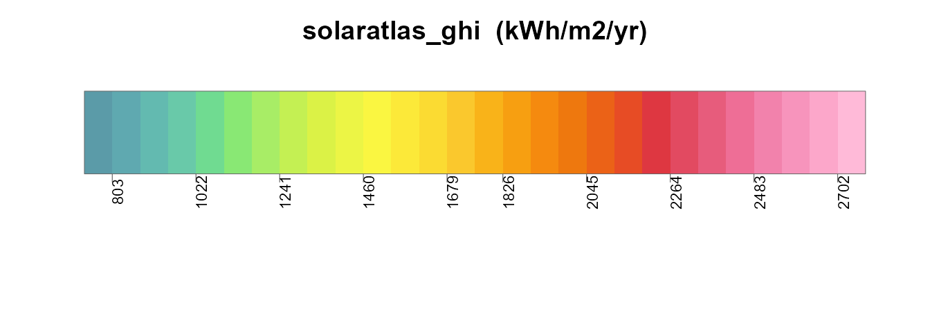
Global Solar Atlas GHI

solaratlas_ghi — family solaratlas, measure ghi, unit kWh/m2/yr
28 stops, 27 breaks from 803 to 2702
Source Global Solar Atlas 2.0 world GHI poster map (World_GHI_poster-map_1500x800mm-300dpi)

Licence CC BY 4.0, with the mandatory WIPO/UNCITRAL dispute-resolution addition in the GSA terms of use

Attribution [Data/information/map] obtained from the Global Solar Atlas 2.0, a free, web-based application developed and operated by the company Solargis s.r.o. on behalf of the World Bank Group, utilizing Solargis data, with funding provided by the Energy Sector Management Assistance Program (ESMAP). For additional information: https://globalsolaratlas.info

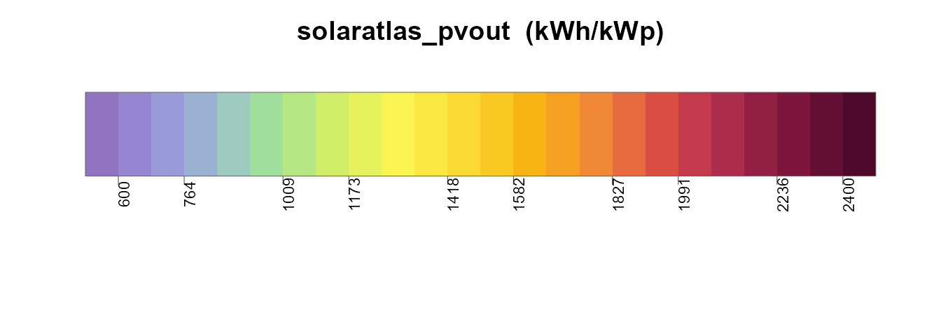
Global Solar Atlas PV output

solaratlas_pvout — family solaratlas, measure pvout, unit kWh/kWp
24 stops, 23 breaks from 600 to 2400
Source Global Solar Atlas 2.0 world PVOUT poster map (World_PVOUT_poster-map_1500x800mm-300dpi)

Licence CC BY 4.0, with the mandatory WIPO/UNCITRAL dispute-resolution addition in the GSA terms of use

Attribution [Data/information/map] obtained from the Global Solar Atlas 2.0, a free, web-based application developed and operated by the company Solargis s.r.o. on behalf of the World Bank Group, utilizing Solargis data, with funding provided by the Energy Sector Management Assistance Program (ESMAP). For additional information: https://globalsolaratlas.info

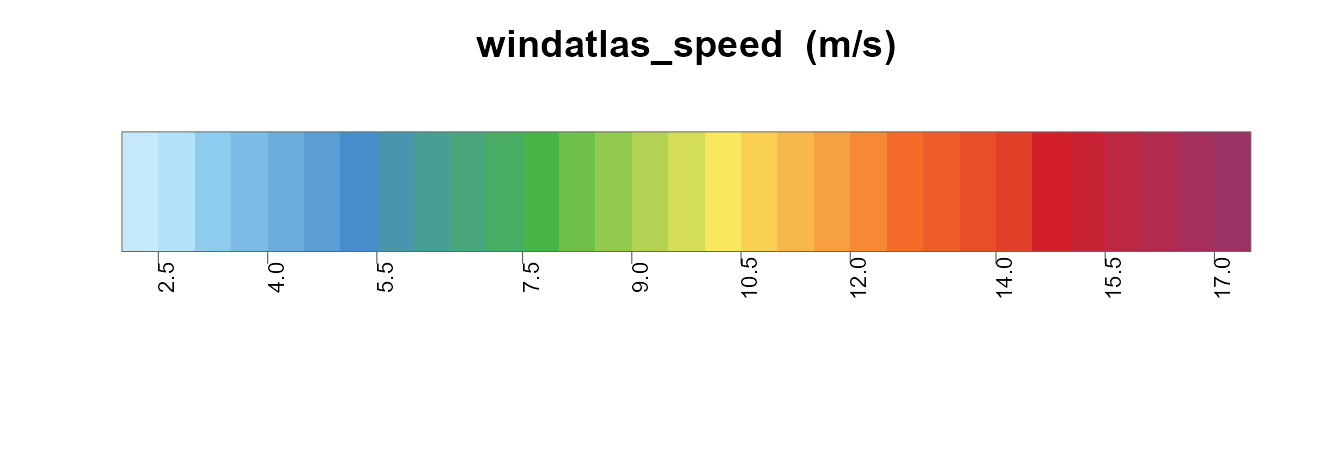
Global Wind Atlas mean wind speed (approximation)

windatlas_speed — family windatlas, measure speed, unit m/s
31 stops, 30 breaks from 2.5 to 17
Source Approximation. Derived from an earlier version of the Global Wind Atlas for the merra2ools package (c. 2020); values recovered by sampling that package’s figure legend, the defining object (palette.windatlas) having been lost. Atlas version unconfirmed and not verified against GWA 3 or 4.

Licence CC BY 4.0 IGO, with the mandatory and binding addition in the GWA terms of use

Attribution [Data/information/map] obtained from the Global Wind Atlas, a free, web-based application developed, owned and operated by the Technical University of Denmark (DTU). The Global Wind Atlas versions 3 and 4 are released in partnership with the World Bank Group, utilizing data provided by Vortex, using funding provided by the Energy Sector Management Assistance Program (ESMAP). Cite The World Bank as the data provider and reference ESMAP as the source of funding.

An atlas publishes several quantities and styles each differently, so each is a separate palette named family_measure. They are not interchangeable. One member of each family is its default, so the bare family name resolves to it:

identical(energypal("windatlas"), energypal("windatlas_speed"))
#> [1] TRUE
energypal_info(family = "windatlas") |> select(name, measure, default, unit)
#>              name measure default unit
#> 1 windatlas_speed   speed    TRUE  m/s

Several measures published by the atlases are not included — wind power density and IEC capacity-factor classes, solar DNI, DIF and GTI — because no verified colour source for them was available, and guessing would defeat the purpose of a store whose value is its provenance. They are better added as one reviewable file each than approximated in bulk.

Orderings

Order carries meaning in energy charts, so palettes declare it rather than leaving it to whatever sequence the file happens to use.

energypal_orders("carriers") |>
  select(order, kind, n, source) |>
  knitr::kable()

order	kind	n	source
carbon_intensity	declared	9	IPCC AR5 WGIII, Annex III, Table A.III.2 (lifecycle medians)
dispatchability	declared	10	IEA World Energy Outlook generation-stack conventions
merit_order	declared	8	Conventional dispatch-stack ordering; indicative only
renewability	declared	10	IEA / IRENA energy-mix chart conventions
spec	computed	93	NA
alpha	computed	93	NA
hue	computed	93	NA
lightness	computed	93	NA
chroma	computed	93	NA

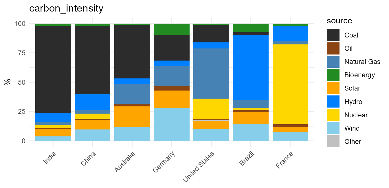
The same data under three of them. The sequence changes; the colour of each carrier does not.

# countries ordered most carbon-intensive first, using the palette's own
# carbon-intensity property - a presentation ordering, not an emissions estimate
latest <- owid_energy_mix |> filter(year == max(year))

# one row per carrier that has a figure: a name can appear twice in the table
# (Nuclear is both a group and the carrier inside it), which would fan the join out
intensity <- energypal_table("carriers") |>
  filter(!is.na(carbon_intensity)) |>
  distinct(carrier = name, carbon_intensity)

rank <- latest |>
  left_join(energypal_match(unique(latest$source), warn = FALSE) |>
              select(source = original, carrier = matched), by = "source") |>
  left_join(intensity, by = "carrier") |>
  group_by(country) |>
  summarise(ci = weighted.mean(carbon_intensity, percentage, na.rm = TRUE)) |>
  arrange(desc(ci))

d <- latest |> mutate(country = factor(country, levels = rank$country))
for (o in c("carbon_intensity", "merit_order", "renewability")) {
  print(
    ggplot(d, aes(country, percentage, fill = source)) +
      geom_col() +
      scale_fill_energy(order = o) +
      labs(title = o, x = NULL, y = "%") +
      theme_minimal() +
      theme(axis.text.x = element_text(angle = 45, hjust = 1))
  )
}

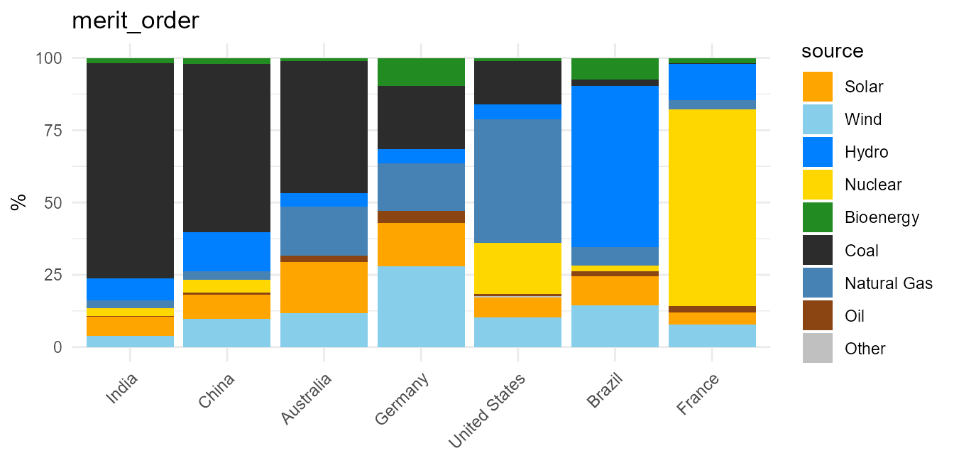
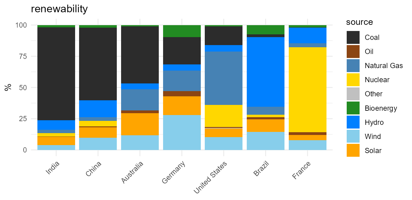
An ordering declared at carrier level covers the subtypes beneath it: an entry the sequence does not name sorts with its nearest named ancestor, so each fuel’s family stays together.

energypal_table("carriers", order = "carbon_intensity") |>
  select(name, type) |>
  head(10)
#>               name    type
#> 1       FossilCoal carrier
#> 2       Anthracite subtype
#> 3       Bituminous subtype
#> 4    SubBituminous subtype
#> 5          Lignite subtype
#> 6             Coke subtype
#> 7  OtherFossilCoal subtype
#> 8        FossilOil carrier
#> 9            Crude subtype
#> 10 ResidualFuelOil subtype

Orderings, and the figures behind them, are for presentation only. They arrange legends and chart series. They are indicative values, not validated figures, and must not be used in calculations. Every declared ordering and numeric property carries a note saying so, which travels with the data:

tab <- energypal_table("carriers")
attr(tab$carbon_intensity, "note")
#> [1] "Presentation only - for ordering and shading. NOT a model input. These are indicative lifecycle medians across a wide reported range; use figures from your own scenario or inventory for any calculation.\n"
attr(tab$carbon_intensity, "source")
#> [1] "IPCC AR5 WGIII, Annex III, Table A.III.2 (lifecycle medians)"

Shades within a carrier

Plant-level data repeats a carrier many times over — a fleet has several coal units and a dozen wind farms. energypal_gradient() spreads one palette colour into distinct tones so those clusters stay apart without losing the fuel.

base <- energypal("carriers", n = 10)
n_sh <- 5

op <- par(mai = c(0.2, 1.15, 0.4, 0.2))
plot.new()
plot.window(xlim = c(0.5, n_sh + 0.5), ylim = c(length(base) + 0.5, 0.5))
for (i in seq_along(base)) {
  sh <- energypal_gradient(base[[i]], n = n_sh)
  for (j in seq_len(n_sh)) {
    rect(j - 0.5, i - 0.42, j + 0.5, i + 0.42, col = sh[j], border = "white", lwd = 0.6)
  }
  mtext(names(base)[i], side = 2, at = i, las = 1, line = 0.3, cex = 0.75)
}
title(main = sprintf("%d shades of each carrier", n_sh), cex.main = 0.95)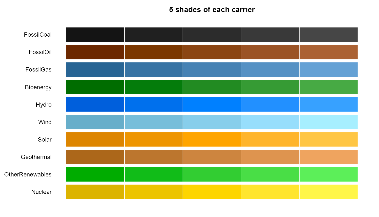

par(op)

The middle column is the palette colour; the gradient spreads symmetrically around it in OKLAB rather than only lightening, which is what keeps a bright carrier like Solar from collapsing to one tone.

energypal_colors(gradient = TRUE) applies this to data, grouping by the carrier each label resolved to:

energypal_colors(c("Coal_1", "Coal_2", "Coal_3", "Wind_N", "Wind_S", "Solar_1"),
                 gradient = TRUE, warn = FALSE)
#>    Coal_1    Coal_2    Coal_3    Wind_N    Wind_S   Solar_1 
#> "#141414" "#2C2C2C" "#464646" "#67AECA" "#A7EFFF" "#FFA500"

Grouping by resolved carrier rather than by colour matters where two entries share a hex code — FossilCoal and OtherFossilCoal are both #2C2C2C, and grouping on the colour would merge them into one gradient.

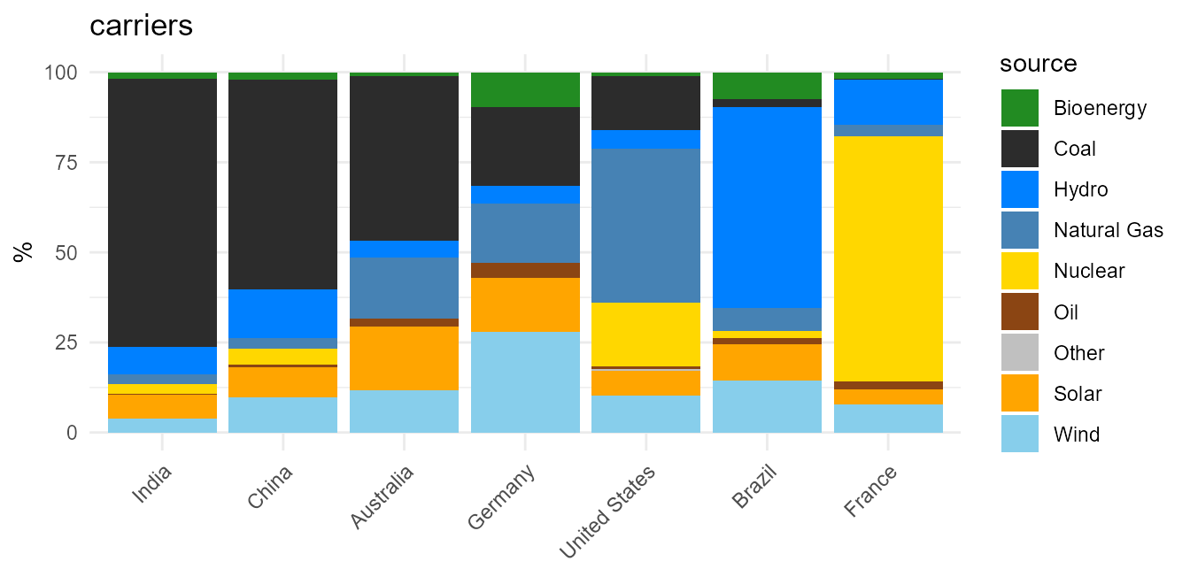
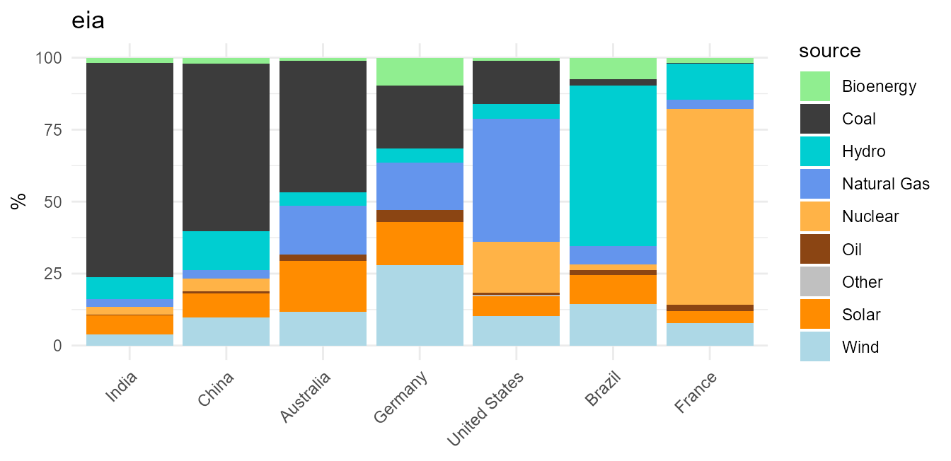
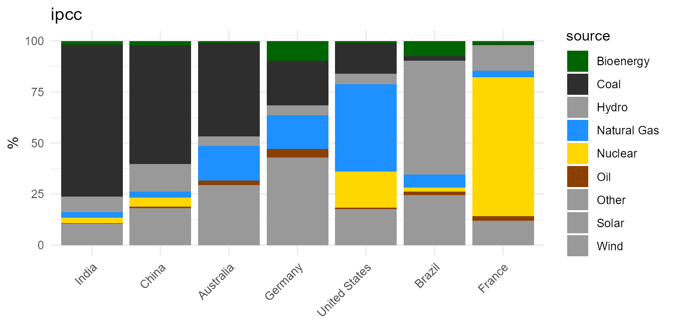
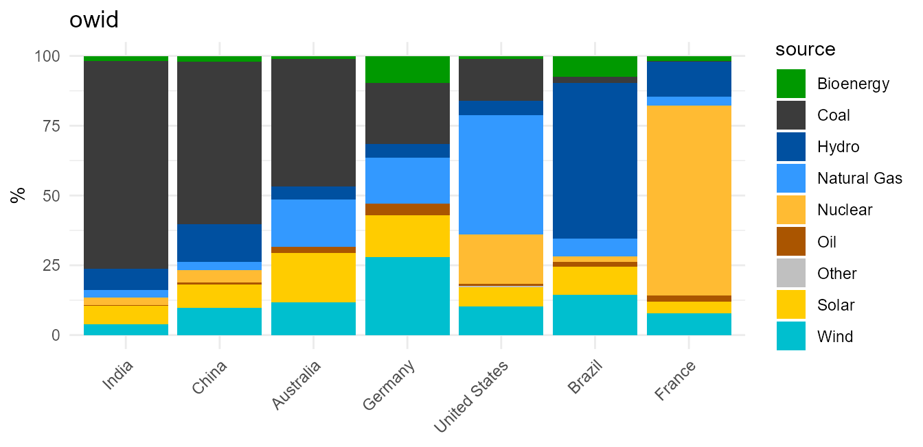
The same chart, four ways

for (p in c("carriers", "eia", "ipcc", "owid")) {
  print(
    ggplot(d, aes(country, percentage, fill = source)) +
      geom_col() +
      scale_fill_energy(palette = p) +
      labs(title = p, x = NULL, y = "%") +
      theme_minimal() +
      theme(axis.text.x = element_text(angle = 45, hjust = 1))
  )
}

Adding a palette

One YAML file in inst/extdata/palettes/, or anywhere on disk if you pass file =. No code changes, no registration in a list, no test edits — the validator tests iterate over the directory, so a new file is picked up and checked automatically.

meta:
  name: myreport
  title: "Colours for the 2026 report"
  source: "Figure 4.2"
  license: "Our own colours"   # required: how they were obtained
  extends: carriers            # optional: inherit labels and aliases
colors:
  FossilCoal: "#3A3A3A"        # state only what this palette publishes
  FossilGas: "#5599CC"

extends applies each entry wherever that name occurs in the parent, at any depth, keeping the labels and aliases it already had — and only those two entries get a colour. A palette that wants to be standalone simply omits it.

f <- tempfile(fileext = ".yml")
writeLines(c("meta:", "  name: myreport", "  license: Our own colours",
             "  extends: carriers",
             "colors:", '  FossilCoal: "#3A3A3A"'), f)

energypal_validate(energypal_spec(file = f))
energypal_colors(c("Coal", "coal power"), file = f)   # aliases inherited
#>       Coal coal power 
#>  "#3A3A3A"  "#3A3A3A"
energypal_colors("Solar", file = f, warn = FALSE)     # not declared here
#>     Solar 
#> "#999999"

Provenance is required

energypal_validate() refuses a palette that does not say where its colours came from, and one declaring a CC BY licence without the citation that licence requires. That rule exists because the store is only worth having if every entry can be traced.

Colours reach a palette one of two ways, and meta.license always says which: reproduced from a downloadable Work published under a licence that permits it — the atlas poster maps — or approximated by eye from a published figure, where the source publishes no colour specification at all. The second is the common case, which is why those palettes are titled (approximation).

Your own palettes are exempt. energypal_register() validates leniently, and energypal_validate(..., strict = FALSE) checks structure alone:

mine <- energypal_create(c(Coal = "#FF0000", Solar = "#00FF00"), name = "mine")
energypal_validate(mine, strict = FALSE)