
Every node of a model renders as LaTeX with as_latex(),
and write_latex() assembles a complete document: sets,
parameters, variables, mappings and equations, with the data summarized
and the folded or trimmed parts annotated. The examples use the small
model built in the Writing a model in R
article.
toy <- example_models$toyEquations and expressions
as_latex(toy$equations$eqDemand)
#> [1] "\\begin{flushleft}\n\\subsection*{\\textbf{eqDemand} -- \\textit{demand is met in every region}} \n\\quad$\\textbf{eqDemand} \n_{\\texttt{region}}$ \n$\\mid\\left\\{\\texttt{region}\\right\\} \\in \\mathit{mR}_{\\texttt{region}}$ \\\\\n\\begin{equation*}\n\\begin{adjustbox}{max width=\\textwidth}\n$\\begin{aligned}\n&\\sum_{\\texttt{tech}} \\bm{\\mathit{vGen}}_{\\texttt{tech},\\texttt{region}} \\ge \\mathsf{pDemand}_{\\texttt{region}} \\\\\n\\end{aligned}$\n\\end{adjustbox}\n\\end{equation*}\n\\vspace{1em}\n\\end{flushleft}"
as_latex(toy$equations$eqCost$rhs)
#> [1] "\\sum_{\\texttt{tech}, \\texttt{region}} \\mathsf{pCapCost}_{\\texttt{tech}}  \\cdot  \\bm{\\mathit{vCap}}_{\\texttt{tech},\\texttt{region}}  +  \\mathsf{pVarCost}_{\\texttt{tech}}  \\cdot  \\bm{\\mathit{vGen}}_{\\texttt{tech},\\texttt{region}}"
Index aliases shorten the subscripts. The toy carries them already
(add_index_aliases() adds them to a model built in R);
write_latex() uses them in equations by default and spells
the full set names in the declarations.
unlist(toy$index_aliases)
#>   tech region
#>    "h"    "r"
A document
write_latex() returns the LaTeX source as a character
vector and, with file =, writes it.
tex <- write_latex(toy)
length(tex)
#> [1] 1
cat(tex[grep("\\\\section", tex)], sep = "\n")
#> \documentclass{article}
#> \usepackage[letterpaper,margin=1in]{geometry}
#> \usepackage{amsmath,amssymb}
#> \usepackage{breqn}
#> \usepackage{graphicx}
#> \usepackage{longtable}
#> \usepackage{adjustbox}
#> \usepackage{multicol}
#> \usepackage{bm}
#> \usepackage[mathcal]{eucal}
#> \usepackage{tikz}
#> \begin{document}
#>
#> \title{Model: toy\\\large two-region capacity expansion toy model}
#> \date{\today}
#> \maketitle
#>
#> \section{Sets}
#> \texttt{region} -- model regions
#>   \quad \textit{(2 elements: north, south)}
#> \\
#> \texttt{tech} -- generation technologies
#>   \quad \textit{(3 elements: coal, gas, wind)}
#> \\
#>
#> \section{Aliases}\
#> \begin{flushleft}
#> \end{flushleft}
#>
#> \section{Index Aliases}\
#> \begin{flushleft}
#> $\texttt{tech} \equiv \texttt{h}$\\
#> $\texttt{region} \equiv \texttt{r}$\\
#> \end{flushleft}
#>
#> \section{Parameters}
#> $\mathsf{pAvail}_{\texttt{tech},\texttt{region}}$ -- availability factor \quad \textit{(6 values)}\\
#> $\mathsf{pCapCost}_{\texttt{tech}}$ -- annualized capacity cost, EUR/kW \quad \textit{(3 values)}\\
#> $\mathsf{pDemand}_{\texttt{region}}$ -- annual demand, MWh \quad \textit{(2 values)}\\
#> $\mathsf{pVarCost}_{\texttt{tech}}$ -- variable cost, EUR/MWh \quad \textit{(3 values)}\\
#>
#> \section{Variables}
#> $\bm{\mathit{vCap}}_{\texttt{tech},\texttt{region}}$ -- installed capacity, kW\\
#> $\bm{\mathit{vCost}}_{}$ -- total system cost, EUR\\
#> $\bm{\mathit{vGen}}_{\texttt{tech},\texttt{region}}$ -- generation, MWh\\
#>
#> \section{Mappings}
#> $\mathit{mR}_{\texttt{region}}$ -- regions \quad \textit{(2 rows)}\\
#> $\mathit{mTR}_{\texttt{tech},\texttt{region}}$ -- technology x region pairs \quad \textit{(6 rows)}\\
#>
#> \section{Equations}\
#> \begin{flushleft}
#> \subsection{\textbf{eqCapLim} -- \textit{generation is limited by available capacity}}
#> \quad$\textbf{eqCapLim}
#> _{\texttt{h},\texttt{r}}$
#> $\mid\left\{\texttt{h},\texttt{r}\right\} \in \mathit{mTR}_{\texttt{tech},\texttt{region}}$ \\
#> \begin{equation*}
#> \begin{adjustbox}{max width=\textwidth}
#> $\begin{aligned}
#> &\bm{\mathit{vGen}}_{\texttt{h},\texttt{r}} \le \mathsf{pAvail}_{\texttt{h},\texttt{r}}  \cdot  \bm{\mathit{vCap}}_{\texttt{h},\texttt{r}} \\
#> \end{aligned}$
#> \end{adjustbox}
#> \end{equation*}
#> \vspace{1em}
#> \end{flushleft}
#>
#>
#> \begin{flushleft}
#> \subsection{\textbf{eqDemand} -- \textit{demand is met in every region}}
#> \quad$\textbf{eqDemand}
#> _{\texttt{r}}$
#> $\mid\left\{\texttt{r}\right\} \in \mathit{mR}_{\texttt{region}}$ \\
#> \begin{equation*}
#> \begin{adjustbox}{max width=\textwidth}
#> $\begin{aligned}
#> &\sum_{\texttt{tech}} \bm{\mathit{vGen}}_{\texttt{h},\texttt{r}} \ge \mathsf{pDemand}_{\texttt{r}} \\
#> \end{aligned}$
#> \end{adjustbox}
#> \end{equation*}
#> \vspace{1em}
#> \end{flushleft}
#>
#>
#> \begin{flushleft}
#> \subsection{\textbf{eqCost} -- \textit{total cost}}
#> \quad$\textbf{eqCost}$
#> \begin{equation*}
#> \begin{adjustbox}{max width=\textwidth}
#> $\begin{aligned}
#> &\bm{\mathit{vCost}}_{} = \sum_{\texttt{tech}, \texttt{region}} \mathsf{pCapCost}_{\texttt{h}}  \cdot  \bm{\mathit{vCap}}_{\texttt{h},\texttt{r}}  +  \mathsf{pVarCost}_{\texttt{h}}  \cdot  \bm{\mathit{vGen}}_{\texttt{h},\texttt{r}} \\
#> \end{aligned}$
#> \end{adjustbox}
#> \end{equation*}
#> \vspace{1em}
#> \end{flushleft}
#>
#>
#>
#> \end{document}
The equations section, one subsection per equation:
i <- grep("subsection\\{\\\\textbf\\{eqDemand", tex)
cat(tex[i:(i + 6)], sep = "\n")
#> \documentclass{article}
#> \usepackage[letterpaper,margin=1in]{geometry}
#> \usepackage{amsmath,amssymb}
#> \usepackage{breqn}
#> \usepackage{graphicx}
#> \usepackage{longtable}
#> \usepackage{adjustbox}
#> \usepackage{multicol}
#> \usepackage{bm}
#> \usepackage[mathcal]{eucal}
#> \usepackage{tikz}
#> \begin{document}
#>
#> \title{Model: toy\\\large two-region capacity expansion toy model}
#> \date{\today}
#> \maketitle
#>
#> \section{Sets}
#> \texttt{region} -- model regions
#>   \quad \textit{(2 elements: north, south)}
#> \\
#> \texttt{tech} -- generation technologies
#>   \quad \textit{(3 elements: coal, gas, wind)}
#> \\
#>
#> \section{Aliases}\
#> \begin{flushleft}
#> \end{flushleft}
#>
#> \section{Index Aliases}\
#> \begin{flushleft}
#> $\texttt{tech} \equiv \texttt{h}$\\
#> $\texttt{region} \equiv \texttt{r}$\\
#> \end{flushleft}
#>
#> \section{Parameters}
#> $\mathsf{pAvail}_{\texttt{tech},\texttt{region}}$ -- availability factor \quad \textit{(6 values)}\\
#> $\mathsf{pCapCost}_{\texttt{tech}}$ -- annualized capacity cost, EUR/kW \quad \textit{(3 values)}\\
#> $\mathsf{pDemand}_{\texttt{region}}$ -- annual demand, MWh \quad \textit{(2 values)}\\
#> $\mathsf{pVarCost}_{\texttt{tech}}$ -- variable cost, EUR/MWh \quad \textit{(3 values)}\\
#>
#> \section{Variables}
#> $\bm{\mathit{vCap}}_{\texttt{tech},\texttt{region}}$ -- installed capacity, kW\\
#> $\bm{\mathit{vCost}}_{}$ -- total system cost, EUR\\
#> $\bm{\mathit{vGen}}_{\texttt{tech},\texttt{region}}$ -- generation, MWh\\
#>
#> \section{Mappings}
#> $\mathit{mR}_{\texttt{region}}$ -- regions \quad \textit{(2 rows)}\\
#> $\mathit{mTR}_{\texttt{tech},\texttt{region}}$ -- technology x region pairs \quad \textit{(6 rows)}\\
#>
#> \section{Equations}\
#> \begin{flushleft}
#> \subsection{\textbf{eqCapLim} -- \textit{generation is limited by available capacity}}
#> \quad$\textbf{eqCapLim}
#> _{\texttt{h},\texttt{r}}$
#> $\mid\left\{\texttt{h},\texttt{r}\right\} \in \mathit{mTR}_{\texttt{tech},\texttt{region}}$ \\
#> \begin{equation*}
#> \begin{adjustbox}{max width=\textwidth}
#> $\begin{aligned}
#> &\bm{\mathit{vGen}}_{\texttt{h},\texttt{r}} \le \mathsf{pAvail}_{\texttt{h},\texttt{r}}  \cdot  \bm{\mathit{vCap}}_{\texttt{h},\texttt{r}} \\
#> \end{aligned}$
#> \end{adjustbox}
#> \end{equation*}
#> \vspace{1em}
#> \end{flushleft}
#>
#>
#> \begin{flushleft}
#> \subsection{\textbf{eqDemand} -- \textit{demand is met in every region}}
#> \quad$\textbf{eqDemand}
#> _{\texttt{r}}$
#> $\mid\left\{\texttt{r}\right\} \in \mathit{mR}_{\texttt{region}}$ \\
#> \begin{equation*}
#> \begin{adjustbox}{max width=\textwidth}
#> $\begin{aligned}
#> &\sum_{\texttt{tech}} \bm{\mathit{vGen}}_{\texttt{h},\texttt{r}} \ge \mathsf{pDemand}_{\texttt{r}} \\
#> \end{aligned}$
#> \end{adjustbox}
#> \end{equation*}
#> \vspace{1em}
#> \end{flushleft}
#>
#>
#> \begin{flushleft}
#> \subsection{\textbf{eqCost} -- \textit{total cost}}
#> \quad$\textbf{eqCost}$
#> \begin{equation*}
#> \begin{adjustbox}{max width=\textwidth}
#> $\begin{aligned}
#> &\bm{\mathit{vCost}}_{} = \sum_{\texttt{tech}, \texttt{region}} \mathsf{pCapCost}_{\texttt{h}}  \cdot  \bm{\mathit{vCap}}_{\texttt{h},\texttt{r}}  +  \mathsf{pVarCost}_{\texttt{h}}  \cdot  \bm{\mathit{vGen}}_{\texttt{h},\texttt{r}} \\
#> \end{aligned}$
#> \end{adjustbox}
#> \end{equation*}
#> \vspace{1em}
#> \end{flushleft}
#>
#>
#>
#> \end{document}
#> NA
#> NA
#> NA
#> NA
#> NA
#> NA
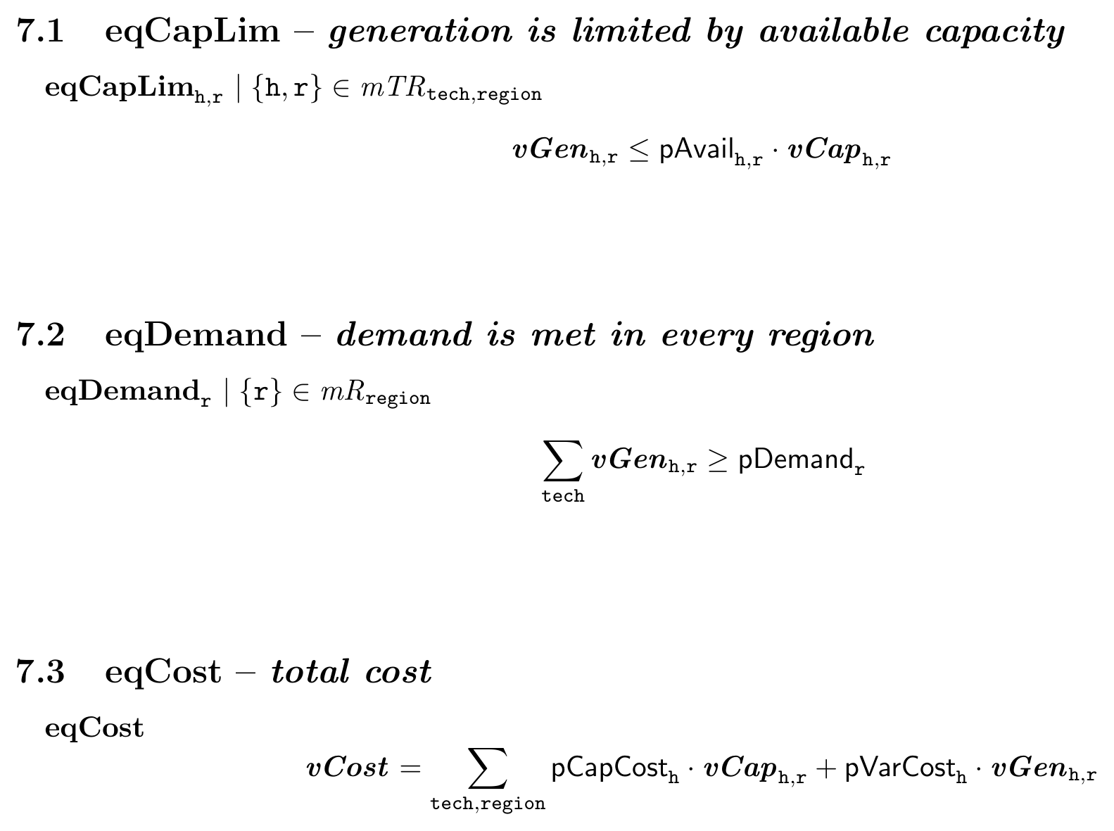
Compiled, the same subsections appear typeset:
Arguments select the sections and the amount of data shown:
tex_eq <- write_latex(toy,
  include_sets = FALSE, include_parameters = FALSE,
  include_variables = FALSE, include_mappings = FALSE,
  include_index_aliases = FALSE
)
length(tex_eq)
#> [1] 1

tex_theory <- write_latex(toy, include_data = FALSE)
length(tex_theory)
#> [1] 1-
include_dataadds set members and parameter row counts;data_detail = "detailed"lists more of each. -
set_display_max_inline,set_display_head_tail_threshold,set_display_head_nandset_display_tail_ncontrol how long sets are abbreviated. -
use_aliases_in_declarations = TRUEuses the short indices in the declarations as well;alias_mapsupplies custom aliases. -
include_toc,title,subtitleandauthorshape the document;preambleandendingreplace the default wrapper.
Folded and trimmed models
A model that has been through fold_model() or
trim_model() (see Folding and
trimming) renders in two views. model_view = "reduced",
the default for such a model, shows the model as it will be solved;
model_view = "full" shows the original declarations with
the folded parameters marked in folded_color and the
trimmed symbols in trimmed_color, plus a summary of what
folding and trimming did.
m <- example_models$energyRt$multimod
mt <- trim_model(m, verbose = FALSE)
get_trim_summary(mt, format = "text")
#> [1] "Model Trimming Summary\n======================\nsets: 6/27 trimmed (22.2%), 21 remaining\nparameters: 1/218 trimmed (0.5%), 217 remaining\nmappings: 160/324 trimmed (49.4%), 164 remaining\nvariables: 10/93 trimmed (10.8%), 83 remaining\nequations: 103/153 trimmed (67.3%), 50 remaining"
tex_full <- write_latex(mt, model_view = "full", trimmed_color = "gray")
sum(grepl("textcolor\\{gray\\}", tex_full))
#> [1] 1
Compiling
The source compiles with pdflatex or xelatex. Its preamble loads
geometry, amsmath, amssymb, breqn, graphicx, longtable, adjustbox,
multicol, bm, eucal and tikz; \textcolor for trimmed
elements comes from xcolor, which tikz loads.
write_latex(toy, file = "toy.tex")
system2("pdflatex", "toy.tex")
The snapshot above is page 2 of that PDF, regenerated with:
write_latex(toy, file = "toy.tex", title = "Model: toy",
            subtitle = "two-region capacity expansion toy model",
            author = "multimod")
tinytex::latexmk("toy.tex", engine = "pdflatex")
page <- magick::image_trim(magick::image_read_pdf("toy.pdf", density = 300)[2])
page <- magick::image_crop(page, paste0(magick::image_info(page)$width, "x1200+0+0"))
magick::image_write(magick::image_border(magick::image_trim(page), "white", "24x24"),
                    "images/toy-latex-rendered.png")
Underscores in symbol names are escaped, and
use_latex_names = TRUE (the default) renders names such as
pCapCost in upright math. Set it to FALSE to
keep every name verbatim.