The data

library(reneuro)
library(dplyr)

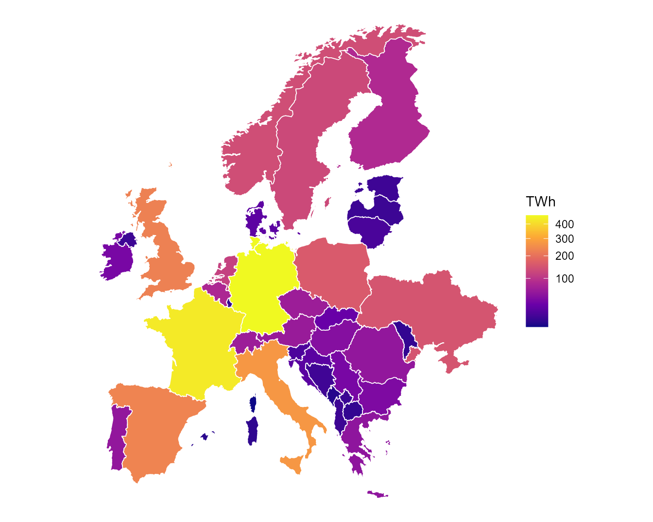
This article uses only shipped data. It needs no PyPSA-Eur clone and no solver.

Three datasets describe the regions the models are built on: nuts_gs (the geography and the data attached to it), nuts_load (demand) and nuts_lines (transmission). Each section below aggregates one of them from NUTS3 to coarser levels and gives the arithmetic used, which differs by quantity: capacities sum, per-capita values take a weighted mean, and peaks and impedances have to be recomputed rather than combined.

1. Geography: five nested levels

gs <- nuts_gs
vapply(geoscales::geoscale_geoframes(gs),
       function(f) length(geoscales::geoscale_regions(gs, f)), 0L)
#> europe  nuts0  nuts1  nuts2  nuts3 
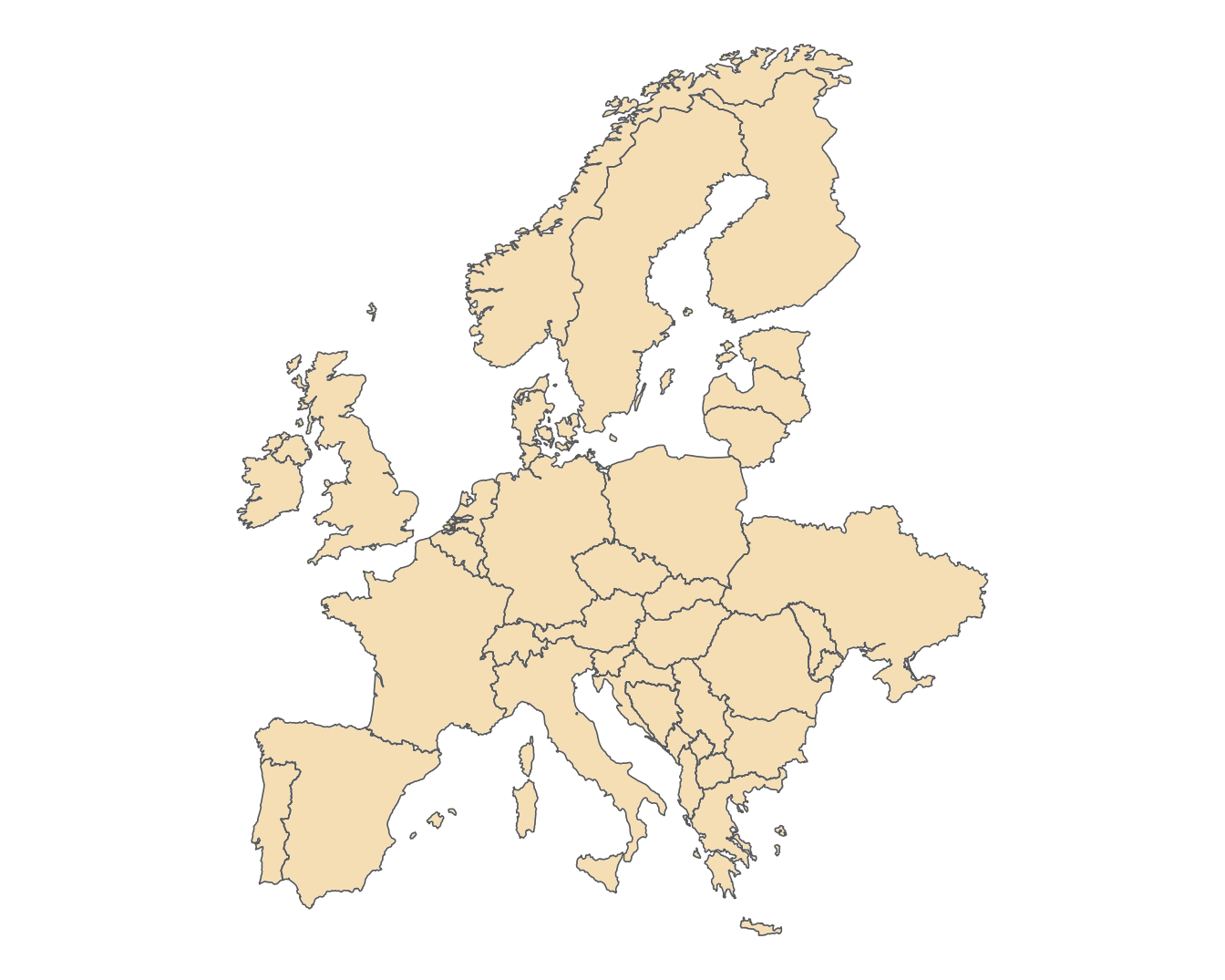
#>      1     36    109    296   1477

1,477 NUTS3 atoms group into 296 NUTS2, 109 NUTS1, 36 countries and a single europe root. Every finer code has exactly one parent; the build asserts this rather than assuming it, and the aggregation below depends on it.

The europe root is the only region at which a continental commodity balance can be declared. newCommodity(geoframe = "europe") gives one Europe-wide CO2 allowance or gas market; without it the coarsest balance is per country, i.e. 36 separate markets.

energyRt::plot_geoscale(gs, type = "stack")

The same hierarchy as an icicle plot:

energyRt::plot_geoscale(gs, type = "icicle") +
  ggplot2::labs(title = NULL)

Four countries — BA, MD, UA, XK — have no NUTS at all and are filled from OpenStreetMap adm1. Those regions become the atoms, and the levels above them are padded (MD0, MD00):

lt <- as.data.frame(geoscales::geoscale_leaftable(gs))

# Every aggregation below is "roll the atoms up to a coarser geoframe", which is
# a lookup from the NUTS3 code to its parent at that level. Named once here
# rather than rebuilt inline each time.
parent_of <- function(level, from = "nuts3") setNames(lt[[level]], lt[[from]])

lt |>
  filter(nuts0 %in% c("BA", "MD", "UA", "XK")) |>
  group_by(nuts0) |>
  summarise(atoms = n(), nuts1 = first(nuts1), nuts2 = first(nuts2))
#> # A tibble: 4 × 4
#>   nuts0 atoms nuts1 nuts2
#>   <chr> <int> <chr> <chr>
#> 1 BA        3 BA0   BA00 
#> 2 MD       37 MD0   MD00 
#> 3 UA       27 UA0   UA00 
#> 4 XK        7 XK0   XK00

PyPSA-Eur repeats the adm1 code at every level, which makes each such region its own parent. The derived hierarchy then contains pairs like (MD-BA, MD-BA), and energyRt’s spatial roll-up becomes vOutTot[MD-BA] = ... + vOutTot[MD-BA], forcing every other term to zero without error.

Eurostat’s convention for identical geography is a distinct code per level: Luxembourg is LU → LU0 → LU00 → LU000, and no NUTS country produces an identity pair. The padding here follows that convention. “NUTS1” and “NUTS2” for these four countries remain stand-ins rather than real administrative levels.

f <- geoscales::geoscale_geoframes(gs)
vapply(seq_len(length(f) - 1L),
       function(i) isTRUE(geoscales::geoscale_nests(gs, f[i], f[i + 1L])),
       logical(1))
#> [1] TRUE TRUE TRUE TRUE

Every adjacent pair nests. Where nesting fails, a region has two parents and its balance is added into both.

2. What each region carries

The leaftable holds 14 data columns per region, in two families. The family determines what a column can be used for.

setdiff(names(lt), c("region", geoscales::geoscale_geoframes(gs)))
#>  [1] "km2"               "pop"               "gdp"              
#>  [4] "gdp_total"         "load_twh"          "peak_mw"          
#>  [7] "n_buses"           "cap_mw"            "hydro_mw"         
#> [10] "pot_onwind"        "pot_solar"         "pot_solar_hsat"   
#> [13] "pot_offwind_ac"    "pot_offwind_dc"    "pot_offwind_float"

Geographic, read from the region shapes and defined for all 1,477 atoms:

column	unit	kind
`km2`	km², equal-area projection	extensive
`pop`	thousands	extensive
`gdp`	EUR per capita	intensive
`gdp_total`	thousand EUR	extensive

Model, read from the NUTS3 network and located at substation buses:

column	unit	kind
`load_twh`	TWh per year	extensive
`peak_mw`	MW, coincident	neither
`n_buses`	substations in the region	extensive
`cap_mw`, `hydro_mw`	MW built today	extensive
`pot_onwind`, `pot_solar`, `pot_solar_hsat`	MW of potential	extensive
`pot_offwind_ac`, `pot_offwind_dc`, `pot_offwind_float`	MW of potential	extensive

Weights

geoscales::geoscale_weights(gs)
#> [1] "km2"        "pop"        "gdp_total"  "load_twh"   "cap_mw"    
#> [6] "pot_onwind" "pot_solar"

A weight splits a coarse quantity across atoms and averages an intensive one back up. Seven columns are declared as weights, and the choice changes the result. German demand split by area differs from the same demand split by population or by measured demand:

de <- filter(lt, nuts0 == "DE")

vapply(c("km2", "pop", "load_twh", "pot_onwind"),
       function(w) round(max(de[[w]]) / sum(de[[w]]), 4), 0)
#>        km2        pop   load_twh pot_onwind 
#>     0.0154     0.0440     0.0312     0.0165

The largest German region takes 1.5% of the country by area and 4.4% by population. No check rejects an unsuitable weight, so the choice is the caller’s to make.

`gdp` is intensive

lt |>
  group_by(nuts0) |>
  summarise(plain_sum = round(sum(gdp)),
            pop_weighted_mean = round(sum(gdp * pop) / sum(pop)),
            gdp_total_bn = round(sum(gdp_total) * 1e3 / 1e9)) |>
  arrange(desc(gdp_total_bn)) |>
  head(5)
#> # A tibble: 5 × 4
#>   nuts0 plain_sum pop_weighted_mean gdp_total_bn
#>   <chr>     <dbl>             <dbl>        <dbl>
#> 1 DE     15618746             41813         3475
#> 2 GB      6887044             37577         2505
#> 3 FR      2963348             36685         2391
#> 4 IT      2929600             30056         1795
#> 5 ES      1239705             26641         1193

Summing gdp over Germany gives 15.6 million, which is not a quantity. The population-weighted mean, ~41,800 EUR, is its GDP per capita. gdp_total is shipped to provide an extensive money weight and gives ~3,475 bn EUR.

The renewable potentials overlap

lt |>
  group_by(nuts0) |>
  summarise(across(c(pot_onwind, pot_solar, pot_solar_hsat,
                     pot_offwind_ac, pot_offwind_dc, pot_offwind_float),
                   \(x) round(sum(x) / 1e3))) |>
  arrange(desc(pot_onwind)) |>
  head(5)
#> # A tibble: 5 × 7
#>   nuts0 pot_onwind pot_solar pot_solar_hsat pot_offwind_ac pot_offwind_dc
#>   <chr>      <dbl>     <dbl>          <dbl>          <dbl>          <dbl>
#> 1 FR           969      1683           1462             30              7
#> 2 SE           942       234            203             64             22
#> 3 ES           938      1095            951             13              0
#> 4 UA           851      3046           2646             62             32
#> 5 NO           790       302            263             45             15
#> # ℹ 1 more variable: pot_offwind_float <dbl>

These columns must not be summed. pot_solar and pot_solar_hsat are fixed-tilt and single-axis-tracking photovoltaics on the same land, and 313 of the 314 offshore regions carry more than one pot_offwind_* type over the same sea area. They ship as separate columns so no summing rule is imposed. The three offshore columns are excluded from the weight set because they are zero for every landlocked country.

Where the model data is zero

lt |>
  summarise(regions = n(),
            no_substation = sum(n_buses == 0),
            pct = round(100 * mean(n_buses == 0), 1))
#>   regions no_substation  pct
#> 1    1477           442 29.9

PyPSA-Eur places demand, plant and potential at substation buses, and 442 NUTS3 regions contain none. Every model column is zero there; the geographic columns are unaffected. The zero reflects the model’s allocation, in which a busless region’s land and load were folded into the neighbour it clusters with, rather than the region itself.

The same applies at coarser levels:

bind_rows(lapply(c("nuts2", "nuts1", "nuts0"), function(l) {
  lt |>
    group_by(group = .data[[l]]) |>
    summarise(buses = sum(n_buses), .groups = "drop") |>
    summarise(level = l, groups = n(), no_substation = sum(buses == 0))
}))
#> # A tibble: 3 × 3
#>   level groups no_substation
#>   <chr>  <int>         <int>
#> 1 nuts2    296             7
#> 2 nuts1    109             3
#> 3 nuts0     36             0

Seven NUTS2 groups and three NUTS1 groups contain no substation. These are the regions lost when 296 NUTS2 regions become 289 model nodes and 109 NUTS1 become 106. A weight summing to zero over a group divides by zero when averaging into it; the affected groups are recorded on the object rather than substituted:

names(attr(gs, "weight_degeneracy"))
#> [1] "load_twh"   "cap_mw"     "pot_onwind" "pot_solar"

Two entries are degenerate for a different reason. GBI3 (Inner London) has no generation and no land the availability rules admit for wind; NO07 (Nord-Norge) has no solar potential, lying above the Arctic Circle.

3. Load

head(nuts_load, 3)
#>    level region    load_twh  peak_gw n_buses
#> 1 europe EUROPE 3356.475513 543.3607    4356
#> 2  nuts0     AL    7.605935   1.6590      13
#> 3  nuts0     AT   69.470957  11.4410      66

Energy is extensive

Going from 1,477 regions to 36 requires only a sum:

Show code

fine <- filter(nuts_load, level == "nuts3")

agg_load <- function(col) {
  fine |>
    mutate(region = parent_of(col)[region]) |>
    group_by(region) |>
    summarise(load_twh = sum(load_twh), .groups = "drop") |>
    mutate(level = col)
}
derived <- bind_rows(lapply(c("nuts0", "nuts1", "nuts2"), agg_load))

# ...and it must agree with what was computed independently at each level.
nuts_load |>
  filter(level %in% c("nuts0", "nuts1", "nuts2")) |>
  select(level, region, load_twh) |>
  inner_join(derived, by = c("level", "region"),
             suffix = c("_shipped", "_derived")) |>
  group_by(level) |>
  summarise(regions = n(),
            max_abs_diff = max(abs(load_twh_derived - load_twh_shipped)))

#> # A tibble: 3 × 3
#>   level regions max_abs_diff
#>   <chr>   <int>        <dbl>
#> 1 nuts0      36     1.42e-14
#> 2 nuts1     109     7.11e-15
#> 3 nuts2     296     7.11e-15

The difference is zero at every level: the parts add to the whole, and no weight is involved.

Peak is not extensive

Show code

pk <- function(fine_lv, coarse_lv) {
  f <- filter(nuts_load, level == fine_lv)
  m <- parent_of(coarse_lv, from = fine_lv)
  tibble(level = coarse_lv,
         summed = sum(tapply(f$peak_gw, m[f$region], sum)),
         coincident = sum(nuts_load$peak_gw[nuts_load$level == coarse_lv]))
}

bind_rows(
  pk("nuts3", "nuts2"), pk("nuts2", "nuts1"), pk("nuts1", "nuts0"),
  tibble(level = "europe",
         summed = sum(nuts_load$peak_gw[nuts_load$level == "nuts0"]),
         coincident = nuts_load$peak_gw[nuts_load$level == "europe"])) |>
  mutate(overstated_pct = round(100 * (summed / coincident - 1), 2))

#> # A tibble: 4 × 4
#>   level  summed coincident overstated_pct
#>   <chr>   <dbl>      <dbl>          <dbl>
#> 1 nuts2    580.       580.           0   
#> 2 nuts1    580.       580.           0   
#> 3 nuts0    580.       580.           0   
#> 4 europe   580.       543.           6.81

In general peak(parent) <= sum(peak(children)), the gap being load diversity. Here the gap is zero within every country and appears only across Europe, at 6.8% (580 GW summed against 543 GW coincident).

This follows from the data rather than from European demand. PyPSA-Eur builds per-bus load as a static fraction times the national hourly series, so every bus in a country has the same normalised shape and their peaks coincide. Diversity appears only where the shapes differ, which is between countries.

Resolution finer than a country therefore adds spatial detail to the level of demand but not to its shape: at NUTS3, 1,477 regions share 36 distinct profiles.

442 regions carry no demand

nuts_load |>
  filter(level == "nuts3") |>
  summarise(regions = n(),
            no_demand = sum(n_buses == 0),
            pct = round(100 * mean(n_buses == 0), 1))
#>   regions no_demand  pct
#> 1    1477       442 29.9

load.substation_only: true places demand only on substation buses, and 442 NUTS3 regions contain none; Germany alone has 182. They ship as explicit zeros rather than missing rows. A NUTS3 model therefore has demand in 70% of its regions, which bounds the resolution that is useful.

The maps

Each region is shaded by its share of its parent’s demand: a country against Europe, a NUTS3 district against the NUTS2 region containing it. Shares of the European total would instead restate the size of each region, which does not change with resolution.

Show the map helpers

library(ggplot2)

# geoscale_geometry() dissolves the atoms up to the requested geoframe and
# returns an sf keyed by it, already carrying the CRS -- so the only work left
# is to give that key column the common name the joins below use.
level_sf <- function(lv) {
  geoscales::geoscale_geometry(nuts_gs, geoframe = lv) |>
    rename_with(\(nm) ifelse(nm == lv, "region", nm))
}

# The geoframes are ordered coarse -> fine, so a level's parent is the one
# before it: nuts3 -> nuts2, and nuts0 -> the single `europe` root.
GF <- geoscales::geoscale_geoframes(nuts_gs)
parent_frame <- function(lv) GF[[which(GF == lv) - 1L]]

load_map <- function(lv) {
  shares <- nuts_load |>
    filter(level == lv) |>
    select(region, load_twh) |>
    left_join(distinct(lt, region = .data[[lv]],
                       parent = .data[[parent_frame(lv)]]), by = "region") |>
    group_by(parent) |>
    # A parent carrying no demand at all divides by zero -- those are the
    # busless groups counted above. They map as missing, not as 0/0.
    mutate(total = sum(load_twh),
           share = if_else(total > 0, 100 * load_twh / total, NA_real_)) |>
    ungroup()

  level_sf(lv) |>
    left_join(select(shares, region, load_twh, share), by = "region")
}
BOX <- list(xlim = c(-11, 32), ylim = c(34, 71))   # crop overseas territories

Show code

# rbind.sf, not bind_rows: the data-frame route drops the CRS and coord_sf()
# then fails inside the projection step.
LEVELS <- c("nuts0", "nuts1", "nuts2", "nuts3")

maps <- do.call(rbind, lapply(LEVELS, function(l) {
  s <- load_map(l); s$level <- l; s
}))
maps$level <- factor(maps$level, levels = LEVELS)

ggplot(maps) +
  geom_sf(aes(fill = share), colour = NA) +
  facet_wrap(~level, ncol = 2) +
  scale_fill_viridis_c(option = "C", trans = "sqrt",
                       name = "% of parent\nregion") +
  coord_sf(xlim = BOX$xlim, ylim = BOX$ylim, expand = FALSE) +
  theme_void() +
  theme(strip.text = element_text(face = "bold"))

At NUTS0 each country’s share of Europe is at most 15%. At NUTS3 the shares spread across the full range: most districts carry a small part of their NUTS2 region and a few carry nearly all of it. The dark patches are the 442 regions with no substation, which carry none. Grey regions are those whose parent has no demand at all — the seven NUTS2 groups counted above.

4. Transmission

nuts_lines holds every base_s line whose ends fall in different NUTS3 regions. The rest were dropped:

p <- attr(nuts_lines, "reneuro_provenance")
c(lines_total = p$lines_total, intra_nuts3_dropped = p$lines_intra_dropped,
  shipped = nrow(nuts_lines))
#>         lines_total intra_nuts3_dropped             shipped 
#>                7360                4218                3142

57% of lines never leave a NUTS3 region, and they carry 53% of the network’s capacity. The finest level available discards more than half the grid.

Aggregating a corridor

Show the aggregation code

centroids <- function(level) {
  s <- level_sf(level)
  cc <- suppressWarnings(sf::st_coordinates(sf::st_centroid(sf::st_geometry(s))))
  tibble(region = s$region, cx = cc[, 1], cy = cc[, 2])
}

haversine <- function(x1, y1, x2, y2) {
  R <- 6371; r <- pi / 180
  a <- sin((y2 - y1) * r / 2)^2 +
       cos(y1 * r) * cos(y2 * r) * sin((x2 - x1) * r / 2)^2
  2 * R * asin(pmin(1, sqrt(a)))
}

agg_lines <- function(level, length_factor = 1.25) {
  m  <- parent_of(level)
  ct <- centroids(level)
  nuts_lines |>
    mutate(f = m[from], t = m[to]) |>
    filter(f != t) |>
    # canonical order, so A-B and B-A are one corridor
    mutate(a = pmin(f, t), b = pmax(f, t)) |>
    left_join(rename(ct, a = region, cx0 = cx, cy0 = cy), by = "a") |>
    left_join(rename(ct, b = region, cx1 = cx, cy1 = cy), by = "b") |>
    mutate(new_len = haversine(cx0, cy0, cx1, cy1) * length_factor,
           lf = if_else(length_km > 0, new_len / length_km, new_len)) |>
    group_by(from = a, to = b) |>
    summarise(s_nom = sum(s_nom), n_lines = n(),
              length_km = first(new_len),
              x = 1 / sum(1 / (lf * x)),        # parallel, length-rescaled
              cx0 = first(cx0), cy0 = first(cy0),
              cx1 = first(cx1), cy1 = first(cy1),
              .groups = "drop")
}

Three rules, taken from pypsa.clustering.spatial:

s_nom sums — thermal ratings of parallel circuits add;
length is recomputed as the great-circle distance between the two region centroids times line_length_factor (1.25) — it is not inherited;
x is rescaled by the length ratio, then parallel-combined as 1 / Σ(1/x).

bind_rows(lapply(LEVELS, function(l) {
  a <- agg_lines(l)
  tibble(level = l, corridors = nrow(a),
         GW = round(sum(a$s_nom) / 1e3),
         median_km = round(median(a$length_km)),
         median_x = round(median(a$x), 2))
}))
#> # A tibble: 4 × 5
#>   level corridors    GW median_km median_x
#>   <chr>     <int> <dbl>     <dbl>    <dbl>
#> 1 nuts0        65   356       459     28.8
#> 2 nuts1       203  1357       253     16.0
#> 3 nuts2       547  2518       154     13.2
#> 4 nuts3      1789  5004        85     11.2

Checked against PyPSA-Eur’s own 41-cluster network, built by its cluster_network rule: the capacity crossing a country boundary sums to 356,352.715 MW there and 356,352.715 MW in the table above. The corridor counts differ (77 against 65) because 41 clusters is not 36 countries. The comparison requires a clone and so is recorded here rather than run.

Note the length column. Aggregating to countries lengthens the network rather than shortening it: a corridor becomes the distance between two national centroids, which for DE–FR spans most of both countries. Impedance follows length, so r rises with it, and since loss ∝ r · s_nom², losses are overestimated at coarse levels.

Capacity is overestimated for a separate reason: summing thermal ratings ignores N-1 security and the loop flows that consume real boundary capacity. PyPSA-Eur compensates with a flat s_max_pu = 0.7, applied identically at 4,382 nodes and at 41.

The two errors act in opposite directions and do not cancel.

The network as the model sees it

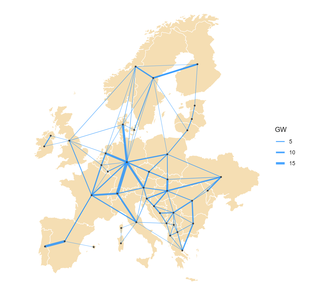
Straight chords between region centroids, which is what the aggregated model contains:

Show code

nets <- bind_rows(lapply(LEVELS, function(l) mutate(agg_lines(l), level = l)))
nets$level <- factor(nets$level, levels = LEVELS)

# white lines alone drown on plasma's bright end -- case them in dark grey
nets$lw <- scales::rescale(nets$s_nom / 1e3, to = c(0.1, 1.4))

ggplot() +
  geom_sf(data = maps, aes(fill = share), colour = NA) +
  geom_segment(data = nets,
               aes(x = cx0, y = cy0, xend = cx1, yend = cy1,
                   linewidth = I(lw + 0.5)),
               colour = "grey15", alpha = 0.85, lineend = "round") +
  geom_segment(data = nets,
               aes(x = cx0, y = cy0, xend = cx1, yend = cy1,
                   linewidth = s_nom / 1e3),
               colour = "white", lineend = "round") +
  facet_wrap(~level, ncol = 2) +
  scale_fill_viridis_c(option = "C", trans = "sqrt", name = "% of parent") +
  scale_linewidth_continuous(range = c(0.1, 1.4), name = "GW") +
  coord_sf(xlim = BOX$xlim, ylim = BOX$ylim, expand = FALSE) +
  theme_void() +
  theme(strip.text = element_text(face = "bold"),
        legend.key = element_rect(fill = "grey35", colour = NA))

At NUTS0 the mesh is reduced to 36 nodes and a small number of long chords. At NUTS3 the structure of the European grid is recognisable, though half of it has already been absorbed into the nodes.

5. Every quantity and its arithmetic

quantity	kind	fine → coarse	coarse → fine
`km2`, `pop`, `gdp_total`	extensive	`sum`	split by weight
`load_twh`, `cap_mw`, `hydro_mw`	extensive	`sum`	split by weight
`pot_*`	extensive	`sum` within a carrier	split by weight
`n_buses`	extensive	`sum`	cannot be split
`gdp` (per capita)	intensive	`weighted_mean` by `pop`	copy
`peak_mw`	neither	cannot be derived — recompute from hourly	—
`s_nom`	extensive	`sum`, intra-region dropped	—
`length`	geometric	recomputed from centroids × 1.25	—
`x`, `r`	reciprocal	rescale by length, then `1/Σ(1/x)`	—
load shape	—	already national; finer adds nothing	—

The kind determines the reduction. Applying the wrong one produces no error: a sum of per-capita GDP, of peaks, or across two overlapping potentials returns a plausible number that does not correspond to any quantity.

1. Geography: five nested levels

2. What each region carries

Weights

gdp is intensive

The renewable potentials overlap

Where the model data is zero

3. Load

Energy is extensive

Peak is not extensive

442 regions carry no demand

The maps

4. Transmission

Aggregating a corridor

The network as the model sees it

5. Every quantity and its arithmetic

See also

`gdp` is intensive