Building a Geoscale from Natural Earth • geoscales

library(geoscales)

The package ships no maps

geoscales contains integration code, not data. There is no data/ directory and no bundled boundaries. A provider fetches a source table; the package records what was fetched.

geo_list_providers()
#>           name                                          desc
#> 1 naturalearth Natural Earth admin-0/admin-1 (rnaturalearth)

Natural Earth is the default provider because its country table is already a wide leaves table — one sf object carries the whole nest as columns:

continent (8) -> region_un -> subregion (22) -> sovereignt
              -> admin / adm0_a3 (177) -> geounit -> subunit

with pop_est and gdp_md as ready-made weights.

gs <- ne_geoscale(scale = 110)
gs
#> Geoscale: naturalearth-110 
#> Description: Natural Earth admin-0 hierarchy 
#> Levels (4, coarsest first):
#>   - continent (8)
#>     - subregion (22)
#>       - country (177)
#>         - feature (177)
#> Atoms: 177
#> Weights: pop_est, gdp_md (default: pop_est)
#> Source: naturalearth
#> Geometry: attached (177 features)

Aggregating up

We will follow Iceland through the hierarchy. It sits in Northern Europe:

lf <- S7::prop(gs, "leaves")
lf[lf$country == "ISL", c("continent", "subregion", "country", "pop_est")]
#>     continent       subregion country pop_est
#> 145    Europe Northern Europe     ISL  361313

Rolling population up from countries to sub-regions is one call. rule = "sum" because population is extensive — it adds up:

pop <- data.frame(country = lf$country, pop = lf$pop_est)
pop <- pop[!is.na(pop$country), ]

agg <- geo_recast(pop, gs, from = "country", to = "subregion", rule = "sum")
agg[agg$subregion == "Northern Europe", ]
#>          subregion       pop
#> 13 Northern Europe 105135601

… and back down

The same verb runs the other way. Going down, rule = "sum" splits a total in proportion to a weight, so the total is conserved:

ne <- agg[agg$subregion == "Northern Europe", ]

back <- geo_recast(ne, gs, from = "subregion", to = "country",
                   rule = "sum", weight = "pop_est")
head(back[order(-back$pop), ], 4)
#>    country      pop
#> 4      GBR 66834405
#> 10     SWE 10285453
#> 1      DNK  5818553
#> 3      FIN  5520314

Because we split by the same quantity we aggregated, the round trip is exact:

back$pop[back$country == "ISL"]
#> [1] 361313
sum(back$pop) == sum(ne$pop)
#> [1] FALSE

That is the whole idea: aggregation and disaggregation are one operation. Direction follows the level ranks, and geo_recast() routes through the atom layer either way.

Iceland’s own regions

Natural Earth’s admin-1 layer gives sub-country units. This needs rnaturalearthhires, which is not on CRAN:

install.packages("rnaturalearthhires",
                 repos = "https://ropensci.r-universe.dev")

s <- ne_source(level = "states", country = "Iceland")
d <- as.data.frame(s)
nrow(d)
#> [1] 9

Nine units — but Iceland has eight regions. Reykjavik and the surrounding capital area are separate admin-1 features that belong to the same region, which Natural Earth records in gn_name. That gives a genuinely ragged hierarchy: one group with two children, seven with one.

isl <- data.frame(
  country    = "ISL",
  landshluti = d$gn_name,       # Iceland's eight regions
  unit       = d$iso_3166_2,    # the nine Natural Earth units
  stringsAsFactors = FALSE
)

g <- geoscale_from_leaves(isl, levels = c("country", "landshluti", "unit"),
                          key = "unit", name = "iceland")
g <- geo_attach_geometry(g, s, by = "iso_3166_2", level = "unit")
g <- geo_area(g, name = "km2")
g
#> Geoscale: iceland 
#> Levels (3, coarsest first):
#>   - country (1)
#>     - landshluti (8)
#>       - unit (9)
#> Atoms: 9
#> Weights: km2 (default: km2)
#> CRS: WGS 84
#> Geometry: attached (9 features)

No level is called region here: geoscale_from_leaves() uses that name for the internal atom key, so it is reserved for the finest level.

The Capital Region is the one that has two units under it:

geo_children(g, "landshluti", "Hofudborgarsvadi")
#> [1] "IS-0" "IS-1"
geo_nests(g, "landshluti", "unit")
#> [1] TRUE

Up: units to regions to country

set.seed(1)
x <- data.frame(unit = geo_regions(g, "unit"),
                generation = round(runif(9, 50, 500)))

geo_recast(x, g, from = "unit", to = "landshluti", rule = "sum")
#>          landshluti generation
#> 1        Austurland        169
#> 2  Hofudborgarsvadi        600
#> 3 Nordurland Eystra        333
#> 4 Nordurland Vestra        347
#> 5         Sudurland        217
#> 6          Sudurnes        308
#> 7        Vestfirdir        475
#> 8        Vesturland        454

geo_recast(x, g, from = "unit", to = "country", rule = "sum")
#>   country generation
#> 1     ISL       2903
sum(x$generation)
#> [1] 2903

Down: a national total split by area

tot <- data.frame(country = "ISL", demand = 1000)

dd <- geo_recast(tot, g, from = "country", to = "unit",
                 rule = "sum", weight = "km2")
dd[order(-dd$demand), ]
#>   unit     demand
#> 9 IS-8 243.839793
#> 7 IS-6 218.218704
#> 8 IS-7 209.284719
#> 6 IS-5 123.058147
#> 5 IS-4  93.745309
#> 4 IS-3  93.738848
#> 3 IS-2   8.612705
#> 2 IS-1   6.034461
#> 1 IS-0   3.467314

Look at what that produces. The Capital Region units receive almost nothing, because they are tiny — yet they hold most of Iceland’s population and would consume most of its electricity. Area is rarely the right weight for demand. This is precisely why geo_recast() makes you name a weight = rather than picking one for you; with a population column on the leaves you would pass that instead.

An intensive quantity must not be summed at all — use weighted_mean, which copies going down and weight-averages going up:

cf <- data.frame(unit = geo_regions(g, "unit"),
                 cf = round(runif(9, 0.2, 0.5), 3))

geo_recast(cf, g, "unit", "landshluti", rule = "weighted_mean", weight = "km2")
#>          landshluti       cf
#> 1        Austurland 0.219000
#> 2  Hofudborgarsvadi 0.348207
#> 3 Nordurland Eystra 0.498000
#> 4 Nordurland Vestra 0.415000
#> 5         Sudurland 0.262000
#> 6          Sudurnes 0.253000
#> 7        Vestfirdir 0.349000
#> 8        Vesturland 0.431000

Geometry follows the levels

geo_geometry() dissolves the atoms up to whatever level you ask for, so the nine units become eight regions:

shp <- geo_geometry(g, level = "landshluti")
nrow(shp)
#> [1] 8

geo_plot(g, level = "landshluti")

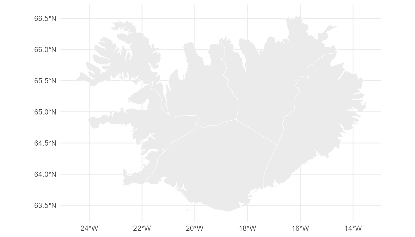
Other providers

The same interface accepts any source. Register one with geo_register_provider(), or pass an sf object straight to geoscale_from_provider(). Natural candidates are giscoR (authoritative NUTS for Europe), geodata/GADM (admin-2 and admin-3 — note its licence forbids commercial use) and tigris (US Census).