Plot a GeoScale

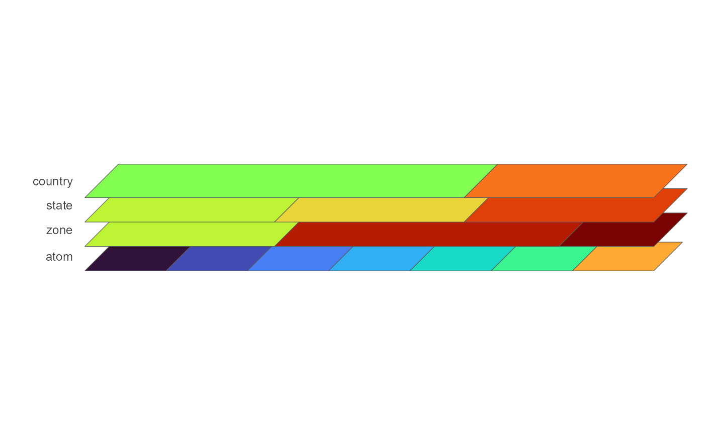
One function for every geoscale figure, selected by type: the structure icicle (default; needs no geometry), the axonometric stack of map planes, and a choropleth map of one geoframe. autoplot() on a GeoScale returns the same ggplot; plot() draws it and returns it invisibly.

Usage

gg_geoscale(
  object,
  type = c("icicle", "stack", "map"),
  data = NULL,
  z = NULL,
  rule = "weighted_mean",
  weight = NULL,
  palette = NULL,
  labels = NULL,
  fill = c("geoframe", "region"),
  geoframe = NULL,
  precision = 0,
  view = NULL,
  angle = NULL,
  ratio = NULL,
  shear = 0.45,
  depth = 0.55,
  gap = NULL,
  rotate = 0,
  direction = c("up", "down"),
  colour = "grey35",
  linewidth = 0.2,
  frame = NULL,
  frame_fill = NA,
  connectors = FALSE,
  outline = NULL,
  outline_colour = "grey20",
  outline_linewidth = 0.6,
  ...
)

# S3 method for class 'GeoScale'
autoplot(object, ...)

# S3 method for class 'GeoScale'
plot(x, ...)

Arguments

object: A GeoScale. The stack and the map need geometry attached with attach_geometry_geoscale() and the sf package.
type: The figure: "icicle" (default), "stack" or "map"; see the sections below. An argument that belongs to another type is an error, not ignored.
data, z: Colour the figure by a value instead of by structure. data is a data.frame with the value column named by z; z is required whenever data is given. The icicle and the stack take data keyed by the atom geoframe and recast the value up to every coarser geoframe (see rule), so the whole figure shares one continuous fill scale; the map takes data keyed by geoframe. Legend title via labs(fill = ).
rule: Icicle and stack, with data: the rule that recasts z from the atoms to each coarser geoframe ("weighted_mean" default; see recast_geoscale()). "share" colours every band or plane by each region's share within the one above it on a fixed linear 0..1 scale; "logshare" is the same on a fixed log10 percent scale.
weight: Icicle and stack: the weight column. On the icicle it sets the rectangle widths; with rule = "weighted_mean" it is also the recast weight. NULL uses the geoscale's default weight.
palette: Fill scale. NULL (default) is the type's own: viridis "H" on the icicle and the stack, ggplot2's default gradient on the map. A viridis option letter ("A".."H") opts into that palette on any type. NA adds no fill scale at all, so a custom one can be supplied, e.g. energypal::scale_fill_energy_b().
labels: What is labelled. NULL (default) is the type's own. Icicle: TRUE (default) draws the region names on the rectangles, FALSE none. Stack: a character vector of geoframes whose regions get their names on the plane (TRUE = all; default none). Map: TRUE draws the region names (default none). Names are the display names of the @meta$labels column where unambiguous, else the codes.
fill: Icicle: what to colour by without data, "geoframe" (default) or "region".
geoframe: Map: the geoframe to draw. Defaults to the atom geoframe.
precision: Stack and map: GEOS precision for the dissolve, forwarded to geoscale_geometry(). Default 0 = off.
view: Stack: a predefined point of view – "oblique" (the shear/depth default), "top-down", "cavalier", "cabinet", "military", "isometric", "dimetric", "trimetric", "perspective" (receding planes shrink) or "pyramid" (receding planes grow: the coarsest geoframe is the small top, the finest the wide base).
angle, ratio: Stack: oblique view by angle (degrees of the receding axis) and foreshortening ratio – e2 = ratio * (cos(angle), sin(angle)). Overridden by view.
shear, depth, gap: Stack: raw receding-axis components (e2 = (shear, depth); used when neither view nor angle/ratio is given) and the vertical spacing between planes: one value for every pair, or one per pair from the top down. gap = NULL (default) spaces planes almost touching, with a slight overlap. Under "perspective" and "pyramid" each spacing is scaled with the planes it separates, so it stays uniform relative to their size.
rotate: Stack: in-plane rotation of each plane (degrees, counter-clockwise).
direction: Stack: "up" (default) stacks the coarsest geoframe on top; "down" puts it at the bottom.
colour, linewidth: Stack: region border colour and width, recycled across the planes (so colour = c("white", "grey40", "white") styles one plane per entry). Defaults "grey35" and 0.2, ggplot2's own sf polygon border.
frame: Stack: draw each plane's outline (the footprint box run through the same projection) as a guide; curved shapes are much easier to read in oblique views with the plane edges visible. TRUE uses "grey80", a colour string uses that colour, NULL (default) draws no frames.
frame_fill: Stack: fill for the plane sheets. Best mostly transparent, e.g. frame_fill = ggplot2::alpha("grey60", 0.12); the panes then read as glass sheets. Setting a fill draws the frames even without frame; NA (default) = no fill.
connectors: Stack: dashed lines joining the corresponding frame corners of adjacent planes, the vertical guides of the stack. TRUE uses the frame colour, a colour string picks its own; default FALSE.
outline: Stack: coarser geoframe(s) whose borders are drawn over every finer plane, so the groups they form are visible at the finer resolution (outline = "zone" marks the zones on the region plane). NULL (default) = none.
outline_colour, outline_linewidth: Stack: colour and width of the outline borders, recycled over outline. Defaults "grey20" and 0.6.
...: Fixed aesthetics for the figure's main layer: the icicle's geom_rect(), the stack's and the map's geom_sf() (e.g. alpha = 0.8).
x: A GeoScale (for plot()).

Value

A ggplot object.

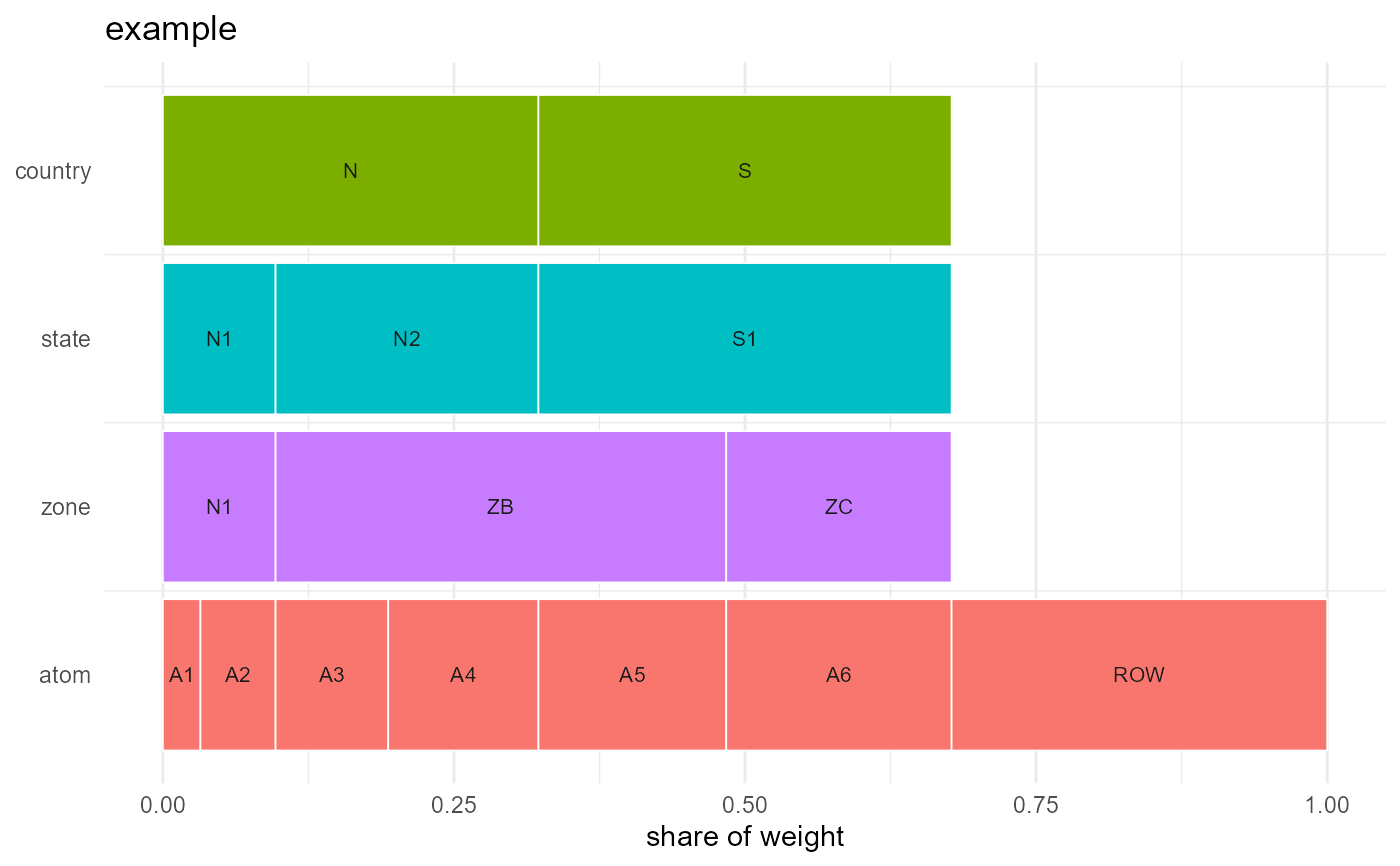
Icicle (`type = "icicle"`)

One row per geoframe, coarsest at the top, each region a rectangle whose width is its share of weight. Shows the GeoScale itself and needs no geometry. With data, each band's rectangles carry the value recast to that geoframe.

Stack (`type = "stack"`)

One sheared map plane per geoframe, coarsest on top: the same atoms dissolved at each resolution, under a chosen point of view. Without data, each plane is coloured by its own regions.

Map (`type = "map"`)

A choropleth of one geoframe. Without data, the region outlines are drawn. Callers that know what their numbers mean (which variable, extensive or intensive, what units) prepare a data.frame keyed by geoframe and hand it here rather than draw their own geom_sf().

Methods

autoplot(object, ...) is gg_geoscale(object, ...). plot(x, ...) prints that figure and returns it invisibly, like base plot().

Examples

if (requireNamespace("ggplot2", quietly = TRUE)) {
  gs <- geoscale_example()
  gg_geoscale(gs)
  ggplot2::autoplot(gs)                           # the same figure
}

if (requireNamespace("ggplot2", quietly = TRUE) &&
    requireNamespace("sf", quietly = TRUE)) {
  # the stack and the map need geometry: one unit square per atom
  gs <- geoscale_example()
  n <- length(geoscale_regions(gs, "atom"))
  square <- function(i) {
    sf::st_polygon(list(cbind(c(i, i + 1, i + 1, i, i), c(0, 0, 1, 1, 0))))
  }
  geom <- do.call(sf::st_sfc, lapply(seq_len(n) - 1, square))
  gs <- attach_geometry_geoscale(gs, geom)
  gg_geoscale(gs, type = "map", geoframe = "state")
  gg_geoscale(gs, type = "stack", view = "cabinet")
}