Geoscale layers for ggplot2 — geom

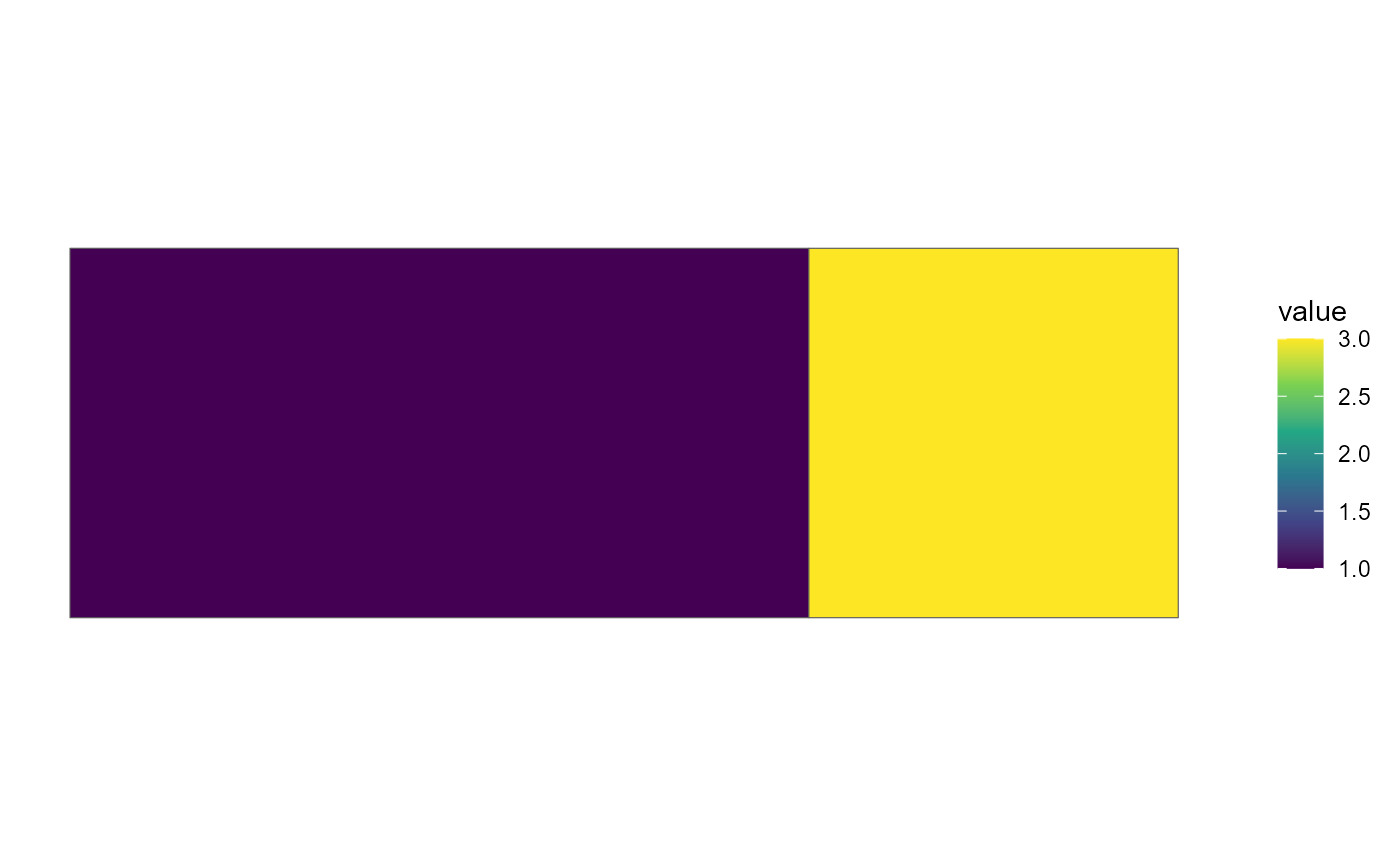
Composable choropleth layers that put region-keyed data on a map inside a normal ggplot() pipeline (the assembled-figure counterparts are geoscale_plot() and geoscale_autoplot()):

Usage

geom_geoscale(
  gs,
  z = NULL,
  geoframe = NULL,
  region = NULL,
  fun = mean,
  data = NULL,
  precision = 0,
  ...
)

theme_geoscale(...)

Arguments

gs: A Geoscale with attached geometry (see attach_geometry_geoscale()).
z: Name of the numeric column of the data to aggregate and fill by; NULL draws plain boundaries.
geoframe: Geoframe to draw. NULL is inferred: the single geoframe name among the data's columns (as in recast_geoscale()), or the atom geoframe when z = NULL.
region: Name of the region-code column of the data. Defaults to the geoframe-named column when present, else "region".
fun: Aggregator collapsing multiple observations per region into one value. Default mean.
data: A data.frame; NULL (default) uses the plot data.
precision: Optional GEOS precision for the dissolve, forwarded to geoscale_geometry(). Default 0 = off.
...: Passed to ggplot2::geom_sf() (e.g. colour, linewidth), or for theme_geoscale() to ggplot2::theme().

Value

A ggplot2::geom_sf() layer (theme_geoscale() returns a theme).

Details

geom_geoscale() — dissolves the object's geometry at geoframe (via geoscale_geometry()), aggregates the value column z per region with fun, and returns a standard ggplot2::geom_sf() layer (with its coord_sf, exactly as geom_sf() does) filled by the aggregated value. With z = NULL it draws plain boundaries.
theme_geoscale() — the quiet map theme: no axes or graticule text, solid white plot background (transparent figures are illegible on dark-mode pages).

The geoscale inputs are column names, not aes() mappings — each call returns one plain sf layer whose data is derived from the plot (or layer) data, so discrete/continuous scales, facets, and themes work through the normal ggplot2 path, and further layers (labels, points) stack on top.

Examples

if (requireNamespace("ggplot2", quietly = TRUE) &&
    requireNamespace("sf", quietly = TRUE)) {
  library(ggplot2)
  sq <- function(x0) sf::st_polygon(list(cbind(
    c(x0, x0 + 1, x0 + 1, x0, x0), c(0, 0, 1, 1, 0))))
  gs <- geoscale_from_leaftable(
    data.frame(state = c("N", "N", "S"), atom = c("a", "b", "c"),
               km2 = c(1, 2, 3)),
    geoframes = c("state", "atom"), name = "toy"
  ) |>
    attach_geometry_geoscale(sf::st_sfc(sq(0), sq(1), sq(2)))

  # data keyed at the drawn geoframe (recast finer data up first)
  ggplot(data.frame(state = c("N", "S"), capacity = c(1, 3))) +
    geom_geoscale(gs = gs, z = "capacity", geoframe = "state") +
    scale_fill_viridis_c() +
    theme_geoscale()
}