Three scales, one vocabulary
A fuel-use table has three dimensions a model cares about: which fuel, where, when. Each is a nested scale – the fuel taxonomy the core ships, and the classes of two sibling packages built on the same core – and each attaches to a table under its own name:
es  <- read_scale("carriers")          # fuels:   group > carrier > fuel
gs  <- geoscale_example()              # regions: country > state > zone > atom
cal <- calendar("m12")                 # time:    MONTH

scale_units(es, "carrier")
#>  [1] "FossilCoal"          "FossilOil"           "FossilGas"
#>  [4] "Bioenergy"           "Hydro"               "Wind"
#>  [7] "Solar"               "Geothermal"          "OtherRenewables"
#> [10] "Nuclear"             "Electricity"         "Heat"
#> [13] "Hydrogen"            "HydrogenDerivatives" "SyntheticFuels"
#> [16] "Storage"             "Other"
geoscale_regions(gs, "country")
#> [1] "N" "S"
calendar_timeslices(cal)
#>  [1] "m01" "m02" "m03" "m04" "m05" "m06" "m07" "m08" "m09" "m10" "m11" "m12"
A fuel-use table
Twelve months of fuel use in six regions for five fuels, in kilotonnes. The numbers are made up but shaped: coal and gas follow a heating season, the size of each region scales its use.
use <- expand.grid(
  atom = geoscale_regions(gs)[geoscale_regions(gs) != "ROW"],
  timeslice = calendar_timeslices(cal),
  fuel = c("Anthracite", "Lignite", "DistillateFuelOil", "NaturalGas",
           "Biodiesel"),
  stringsAsFactors = FALSE
)
base <- c(Anthracite = 2, Lignite = 6, DistillateFuelOil = 1.5,
          NaturalGas = 4, Biodiesel = 0.3)
seasonal <- c(Anthracite = 0.6, Lignite = 0.6, DistillateFuelOil = 0.1,
              NaturalGas = 0.8, Biodiesel = 0)
size <- geoscale_leaftable(gs) |>
  transmute(atom, size = km2 / mean(km2))
use <- use |>
  left_join(size, by = "atom") |>
  mutate(
    month = match(timeslice, calendar_timeslices(cal)),
    kt = base[fuel] * size *
      (1 + seasonal[fuel] * cos(2 * pi * (month - 1) / 12))
  ) |>
  select(atom, timeslice, fuel, kt)
head(use)
#>   atom timeslice       fuel        kt
#> 1   A1       m01 Anthracite 0.7225806
#> 2   A2       m01 Anthracite 1.4451613
#> 3   A3       m01 Anthracite 2.1677419
#> 4   A4       m01 Anthracite 2.8903226
#> 5   A5       m01 Anthracite 3.6129032
#> 6   A6       m01 Anthracite 4.3354839
Attach all three
Each join adds columns prefixed by the scale’s name, so the three never collide and a reader can see which scale a column came from:
labelled <- use |>
  join_scale(es, frame = "fuel", attach = TRUE) |>
  join_geoscale(gs = gs, geoframe = "atom", geoframes = TRUE) |>
  join_calendar(calendar = cal, meta = TRUE)
names(labelled)
#>  [1] "atom"             "timeslice"        "fuel"             "kt"
#>  [5] "carriers.group"   "carriers.carrier" "carriers"         "example.country"
#>  [9] "example.state"    "example.zone"     "example"          "m12"
#> [13] "m12.share"        "m12.weight"
head(labelled, 3)
#>   atom timeslice       fuel        kt carriers.group carriers.carrier
#> 1   A1       m01 Anthracite 0.7225806    FossilFuels       FossilCoal
#> 2   A2       m01 Anthracite 1.4451613    FossilFuels       FossilCoal
#> 3   A3       m01 Anthracite 2.1677419    FossilFuels       FossilCoal
#>     carriers example.country example.state example.zone example m12  m12.share
#> 1 Anthracite               N            N1           N1      A1 m01 0.08493151
#> 2 Anthracite               N            N1           N1      A2 m01 0.08493151
#> 3 Anthracite               N            N2           ZB      A3 m01 0.08493151
#>   m12.weight
#> 1        744
#> 2        744
#> 3        744
carriers.carrier and carriers.group come
from the fuel scale, example.country and friends from the
GeoScale, m12.share and m12.weight (hours)
from the Calendar.
Mass to energy to CO2
The fuel scale carries the IPCC 2006 net calorific value (GJ/t) and CO2 factor (kg/TJ) for these five fuels. Each conversion is one call, keyed by fuel, and the factor applied is reported alongside the result:
energy <- use |>
  mutate(t = kt * 1e3) |>
  select(atom, timeslice, fuel, t) |>
  convert_scale(es, "lhv", from_unit = "t", to_unit = "GJ") |>
  transmute(atom, timeslice, fuel, tj = t / 1e3)

co2 <- energy |>
  convert_scale(es, "ef_co2", from_unit = "TJ", to_unit = "kg") |>
  rename(kg_co2 = tj) |>                 # the converted column: kg CO2
  transmute(atom, timeslice, fuel, tj = energy$tj, kt_co2 = kg_co2 / 1e6)
head(co2, 3)
#>   atom timeslice       fuel       tj   kt_co2
#> 1   A1       m01 Anthracite 19.29290 1.896492
#> 2   A2       m01 Anthracite 38.58581 3.792985
#> 3   A3       m01 Anthracite 57.87871 5.689477
Aggregate along any dimension
Every scale aggregates with the same verb and the same rules. Columns the scale does not know (the other dimensions’ keys) are carried through as identifiers. One registration covers all three dimensions:
register_scale_rule("tj", "sum")
register_scale_rule("kt_co2", "sum")
By carrier and month – the fuel dimension collapses, region and month stay:
by_carrier <- co2 |>
  recast_scale(es, source = "fuel", target = "carrier",
               missing_sources = "ignore") |>
  filter(!is.na(tj))
#> Warning: 66 source unit(s) present in the scale but missing from the data (e.g.
#> Ammonia, AssociatedGas, Battery, ... (66 total)); produced NAs
head(by_carrier, 3)
#>      carrier atom timeslice       tj   kt_co2
#> 1 FossilCoal   A1       m01 45.08903 4.501901
#> 2  FossilOil   A1       m01 16.02097 1.187154
#> 3  FossilGas   A1       m01 78.03871 4.377972
sum(by_carrier$tj) - sum(co2$tj)
#> [1] 0
The table reports five of the 71 fuels. With
missing_sources = "ignore" the others count as unused
rather than unknown, and the total is conserved – the difference above
is zero.
By country – the pipeline verb recast()
dispatches on whichever scale it is handed, so the two aggregations
chain:
by_country <- co2 |>
  recast(es, target = "carrier", missing_sources = "ignore") |>
  filter(!is.na(tj)) |>
  recast(gs, target = "country")
#> Warning: 66 source unit(s) present in the scale but missing from the data (e.g.
#> Ammonia, AssociatedGas, Battery, ... (66 total)); produced NAs
by_country |>
  group_by(country) |>
  summarise(tj = sum(tj), kt_co2 = sum(kt_co2))
#> # A tibble: 2 × 3
#>   country     tj kt_co2
#>   <chr>    <dbl>  <dbl>
#> 1 N       10551.   775.
#> 2 S       11607.   852.
By quarter – a calendar recast needs the year, to place the months on real dates:
by_quarter <- by_carrier |>
  select(carrier, atom, timeslice, tj, kt_co2) |>
  recast_calendar(source = cal, target = calendar("q4"), year = 2024)
head(by_quarter, 4)
#>   timeslice    carrier atom        tj    kt_co2
#> 1        Q1 FossilCoal   A1 124.54761 12.435420
#> 2        Q2 FossilCoal   A1  61.44465  6.134923
#> 3        Q3 FossilCoal   A1  44.53626  4.446710
#> 4        Q4 FossilCoal   A1 107.63922 10.747207
sum(by_quarter$tj) - sum(by_carrier$tj)
#> [1] 0
Draw it with energypal’s colours
energypal’s carriers palette is the same taxonomy, so
the carrier ids map straight onto its colours with no relabelling:
by_carrier |>
  group_by(timeslice, carrier) |>
  summarise(tj = sum(tj), .groups = "drop") |>
  ggplot(aes(x = timeslice, y = tj, fill = carrier)) +
  geom_col() +
  energypal::scale_fill_energy(palette = "carriers",
                               label_style = "short") +
  labs(x = NULL, y = "TJ", fill = NULL,
       title = "Energy use by month and carrier") +
  theme_minimal()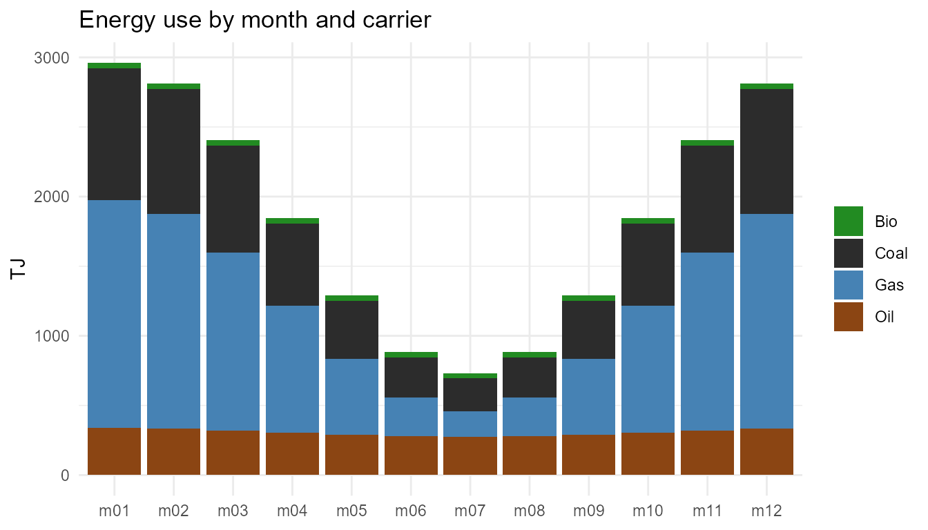
by_country |>
  group_by(country, carrier) |>
  summarise(kt_co2 = sum(kt_co2), .groups = "drop") |>
  ggplot(aes(x = country, y = kt_co2, fill = carrier)) +
  geom_col() +
  energypal::scale_fill_energy(palette = "carriers",
                               label_style = "short") +
  labs(x = NULL, y = "kt CO2", fill = NULL,
       title = "CO2 by country and carrier") +
  theme_minimal()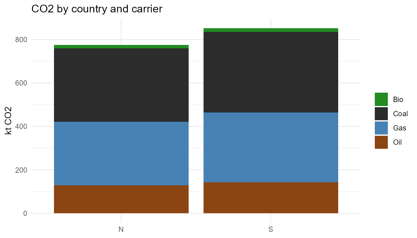
The GeoScale draws its own hierarchy with data attached – CO2 summed to every geoframe at once:
co2_by_atom <- co2 |>
  group_by(atom) |>
  summarise(kt_co2 = sum(kt_co2), .groups = "drop")
geoscale_autoplot(gs, data = co2_by_atom, z = "kt_co2", rule = "sum")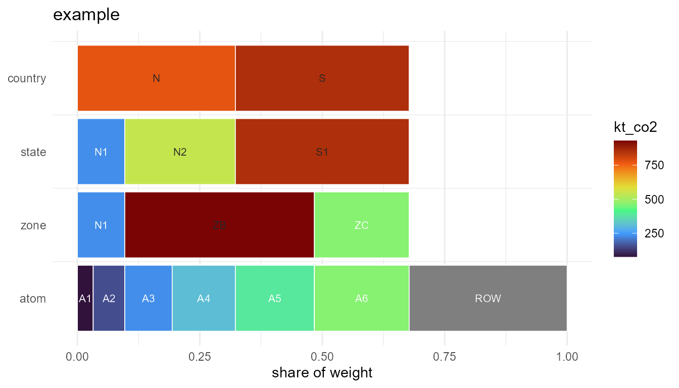
Matching labels from a statistical source
Real sources spell carriers their own way. energypal ships a slice of
Our World in Data’s electricity mix; its source labels
resolve against the fuel scale’s names and aliases exactly, with
frame = "carrier" settling the names that exist at two
frames (Nuclear, Other):
mix <- energypal::owid_energy_mix
matched <- scale_match(es, unique(mix$source), frame = "carrier")
matched
#>         label   frame       unit method candidates
#> 1   Bioenergy carrier  Bioenergy  exact       <NA>
#> 2        Coal carrier FossilCoal  alias       <NA>
#> 3       Hydro carrier      Hydro  exact       <NA>
#> 4 Natural Gas carrier  FossilGas  alias       <NA>
#> 5     Nuclear carrier    Nuclear  exact       <NA>
#> 6         Oil carrier  FossilOil  alias       <NA>
#> 7       Solar carrier      Solar  exact       <NA>
#> 8        Wind carrier       Wind  exact       <NA>
#> 9       Other carrier      Other  exact       <NA>
Join the resolved id on and the palette applies:
mix |>
  filter(year == 2024) |>
  left_join(matched |> select(source = label, carrier = unit),
            by = "source") |>
  ggplot(aes(x = country, y = generation_twh, fill = carrier)) +
  geom_col(position = "fill") +
  energypal::scale_fill_energy(palette = "carriers",
                               label_style = "short") +
  labs(x = NULL, y = "share of generation", fill = NULL,
       title = "Electricity generation mix, 2024 (OWID)") +
  theme_minimal()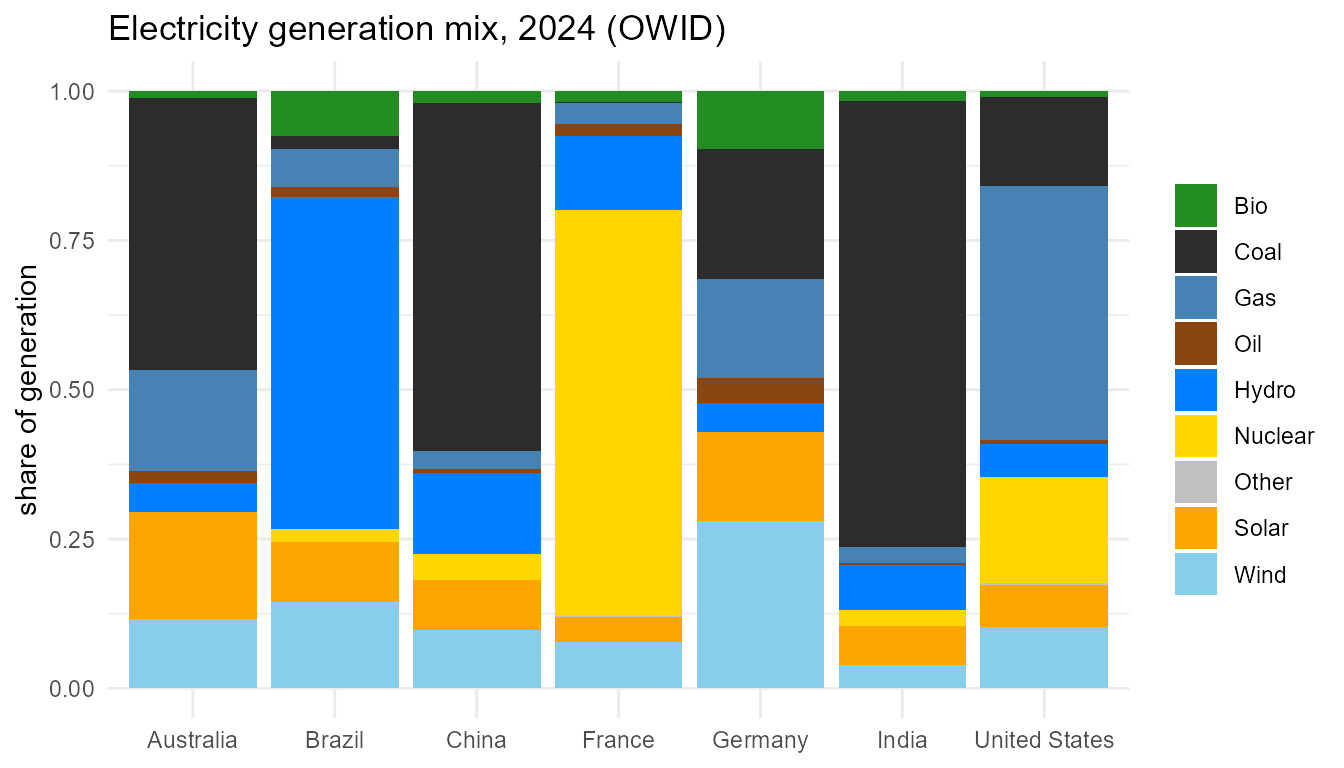
What each package did
| package | contributed | |
|---|---|---|
| fuels | nestedscales (carriers) |
the taxonomy, calorific values, CO2 factors, label matching |
| regions | geoscales | the region hierarchy, aggregation to countries, the icicle |
| time | timescales | month shares and hours, aggregation to quarters |
| colours | energypal | one palette for every figure, by carrier id |
The core is what lets one table carry all three and lets
recast() chain across them.