Plot a calendar's structure as an icicle — calendar

One horizontal band per timeframe (ANNUAL root on top, coarsest first), rectangle widths proportional to timeslice shares, x spanning the covered year on [0, 1]. autoplot() and plot() on a Calendar dispatch here.

Usage

calendar_autoplot(
  x,
  type = c("icicle", "stack"),
  fill = c("order", "share", "weight"),
  color_pattern = c("within", "global"),
  labels = c("name", "timeslice", "none"),
  max_labels = 60L,
  max_segments = 2000L,
  border = NA,
  palette = "D",
  annual = TRUE,
  view = NULL,
  angle = NULL,
  ratio = NULL,
  shear = 0.5,
  depth = 0.3,
  gap = NULL,
  rotate = 0,
  direction = c("up", "down"),
  colour = "grey35",
  linewidth = 0.2,
  frame = NULL,
  frame_fill = NA,
  connectors = FALSE,
  data = NULL,
  z = NULL,
  rule = "weighted_mean",
  year = NULL,
  by = "hour",
  ...
)

# S3 method for class 'Calendar'
autoplot(object, ...)

# S3 method for class 'Calendar'
plot(x, ...)

Arguments

x: A Calendar (for plot()).
type: "icicle" (default) or "stack" — the axonometric stacked-planes view (see below).
fill: What drives the fill gradient: "order" (chronological position, default), "share", or "weight".
color_pattern: For fill = "order": "within" (default) restarts the gradient inside each parent timeslice (hours recycle every day); "global" sweeps once across the whole year.
labels: Segment labels. Icicle: "name" (level value, e.g. h00; default), "timeslice" (full path, e.g. Q1_h00), or "none"; TRUE/FALSE are accepted as shorthands. type = "stack": a character vector of timeframes whose member names are drawn on their plane's segments (e.g. labels = "SEASON"); unset = none.
max_labels: Rows with more segments than this get no labels. Default 60.
max_segments: Rows with more segments than this are binned by x-midpoint before drawing (fill = width-weighted mean), keeping hourly calendars fast. Default 2000.
border: Rectangle border color. Default NA (none), so dense rows render as smooth gradients.
palette: Viridis option letter or name ("D"/"viridis", "C"/"plasma", "B", "A", "E", "turbo"...). Default "D". type = "stack" also accepts NULL: no fill scale is added, so you can supply your own (e.g. an energypal scale).
annual: Include the ANNUAL root band. Default TRUE.
view: type = "stack" only: a predefined point of view – "oblique" (the shear/depth default), "top-down", "cavalier", "cabinet", "military", "isometric", "dimetric", "trimetric", or "perspective" (receding planes shrink).
angle, ratio: type = "stack" only: oblique view by angle (degrees of the receding axis) and foreshortening ratio – e2 = ratio * (cos(angle), sin(angle)). Overridden by view.
shear, depth, gap: type = "stack" only: the raw receding-axis components (e2 = (shear, depth); used when neither view nor angle/ratio is given) and the vertical spacing between planes. gap = NULL (default) spaces planes almost touching, with a slight overlap (0.85 x the plane's screen height).
rotate: type = "stack" only: in-plane rotation of each plane (degrees, counter-clockwise) before projection.
direction: type = "stack" only: "up" (default) stacks the coarsest timeframe on top; "down" puts it at the bottom.
colour, linewidth: type = "stack" only: segment border colour and width, recycled across the planes (one entry per plane styles them individually). Defaults "grey35" and 0.2 – ggplot2's own sf polygon border. (The icicle's rectangle border is the separate border argument.)
frame: type = "stack" only: draw each plane's outline (the unit box run through the same projection) as a guide. TRUE uses "grey80", a colour string uses that colour, NULL (default) draws no frames.
frame_fill: type = "stack" only: fill for the plane sheets; best mostly transparent, e.g. frame_fill = ggplot2::alpha("grey60", 0.12). Setting a fill draws the frames even without frame; NA (default) = no fill.
connectors: type = "stack" only: dashed lines joining the corresponding frame corners of adjacent planes. TRUE uses the frame colour, a colour string picks its own; default FALSE.
data, z: Colour the figure by a value instead of by structure: works for BOTH types – the icicle fills each band's rectangles, the stack fills each plane. data is a data.frame with a timeslice column at the calendar's resolution (or a calendar-named label column) plus the value column named by z; every timeframe gets the value recast to its resolution, so the whole figure shares one continuous fill scale (legend title via labs(fill = )). On the icicle, data overrides fill/color_pattern, and dense bands are binned with width-weighted means.
rule: With data: aggregation rule for the per-timeframe recasts ("sum", "mean", "weighted_mean", ... – see recast_calendar(); explicit or registered, never guessed).
year: With data: the model year the recast routes through (required by recast_calendar()).
by: With data: base-grid granularity for the per-timeframe recasts. Defaults to "hour" – always correct (the automatic choice can pick a daily grid for sub-daily calendars, which silently collapses hour-type slices).
...: Passed on to calendar_autoplot().
object: A Calendar (the S3 autoplot() generic's argument name; calendar_autoplot() itself takes x).

Value

A ggplot object (returned, not printed).

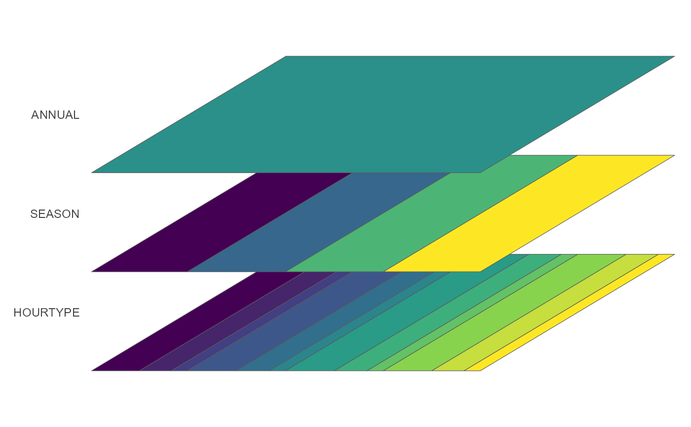
The stack view

type = "stack" draws the same structure axonometrically — one sheared plane per timeframe, ANNUAL on top, each plane segmented by the true duration shares, with segments visibly nesting into the plane above. fill/labels/max_segments apply to the icicle only; the stack colours each plane by its own segment order.

Examples

if (requireNamespace("ggplot2", quietly = TRUE)) {
  calendar_autoplot(calendar("q4_h24"))
  ggplot2::autoplot(calendar("m12"))   # same via the generic
  calendar_autoplot(calendar("s4_hp3"), type = "stack")
}