What problem does this solve?
Energy-system, climate, and operations models all carve the year into discrete timeslices. Different models pick different slicings: 365 days, 12 months, 4 quarters × 24 hours, 168 hours of a representative week, and so on. The timeslice labels are arbitrary, the shares of a year are model-defined, and converting data between slicings is error-prone.
timescales represents any such slicing as a
Calendar: an ordered hierarchy of timeframes
(YEAR, MONTH, HOUR, …) whose
finest nodes — enumerated in the @leaftable — are the
timeslices. With one object you get:
- a stable schema for the timeslice labels and their year-share weights,
- well-defined mappings to and from real datetimes,
- well-defined conversions between any two calendars covering the same year fraction,
- ggplot2-ready visualization, from heatmap layers to wall calendars.
A 5-minute tour
1. Build a calendar
The fastest path uses token-based names — 43 curated
designs ship in the catalog (calendar_catalog()), from
d365_h24 down to typical-period compressions, including the
April-anchored fiscal family (calendar("fy04_m12") — Indian
reporting years):
cal_my <- calendar("m12_h24")    # 12 months × 24 hours = 288 timeslices
cal_my
#> Calendar: m12_h24
#> Timeframes (2):
#>   - MONTH (12) [token: m12]
#>   - HOUR (24) [token: h24]
#> Leaf timeslices: 288
#> year_fraction: 1
#> year_start: month=1, day=1
#> utc_offset_minutes: 0
Equivalent declarative form:
cal_my2 <- calendar_build("m12", "h24")
identical(cal_my@timeframes, cal_my2@timeframes)
#> [1] TRUE
For full control there is the lowest-level constructor
calendar_from_leaftable(), where you supply the leaves
table directly.
2. Inspect the structure
A Calendar has four parts:
cal_my@timeframes               # the timeframe hierarchy, coarsest first
#> [1] "MONTH" "HOUR"
head(calendar_leaftable(cal_my), 4)          # the leaf table (one row per timeslice)
#>   MONTH HOUR       share weight timeslice
#> 1   m01  h00 0.003538813     31   m01_h00
#> 2   m02  h00 0.003196347     28   m02_h00
#> 3   m03  h00 0.003538813     31   m03_h00
#> 4   m04  h00 0.003424658     30   m04_h00
cal_my@members$MONTH             # ordered label vocabulary per timeframe
#>  [1] "m01" "m02" "m03" "m04" "m05" "m06" "m07" "m08" "m09" "m10" "m11" "m12"
cal_my@meta[c("name", "year_fraction")]
#> $name
#> [1] "m12_h24"
#>
#> $year_fraction
#> [1] 1
@leaftable is a plain data.frame. Each row
is one timeslice, with columns:
-
timeslice— the unique timeslice ID, -
share— fraction of a year, -
weight— timeslice weight in hours (defaultshare * 8760), - one column per timeframe — the member label at that level.
3. Map real datetimes onto the calendar
times <- as.POSIXct(c("2025-01-15 03:00", "2025-07-20 18:00"), tz = "UTC")
datetime_to_timeslice(times, cal_my)
#> [1] "m01_h03" "m07_h18"
4. Convert data between calendars
Suppose you have monthly load values and need quarterly averages:
cal_m <- calendar("m12")
cal_q <- calendar("q4")

monthly <- data.frame(
  timeslice = sprintf("m%02d", 1:12),
  load  = c(120, 118, 105,  92,  85,  88,  95, 100,  98,  90, 105, 122)
)

recast_calendar(monthly, from = cal_m, to = cal_q, year = 2025,
       rule = "weighted_mean", by = "day")
#>   timeslice      load
#> 1        Q1 114.21111
#> 2        Q2  88.29670
#> 3        Q3  97.66304
#> 4        Q4 105.67391
The result is day-weighted: Q1 = (31·v₁ + 28·v₂ + 31·v₃) / 90. The
rule is deliberately mandatory — pass one, or register it
per column with register_calendar_rule(); a silently
guessed rule would be a silent unit error. join_calendar()
is the lighter companion: it attaches a calendar’s labels and
timeframe columns to a dataset instead of converting it.
5. Visualize
Every figure tier works through normal ggplot2 — a heatmap layer
here; wall calendars, profiles, duration curves, and the data-filled
structure figures (icicles and stacks take
data =/z =) in
vignette("visualization"):
library(ggplot2)
x <- data.frame(timeslice = calendar_leaftable(cal_my)$timeslice)
x$load <- 80 + 40 * sin(seq(0, 6 * pi, length.out = nrow(x)))
ggplot(x) +
  geom_calendar_tile(calendar = cal_my, z = "load") +
  scale_fill_viridis_c(option = "H") +
  scale_y_discrete(breaks = calendar_breaks()) +
  labs(x = "month", y = "hour", fill = "load") +
  theme_calendar()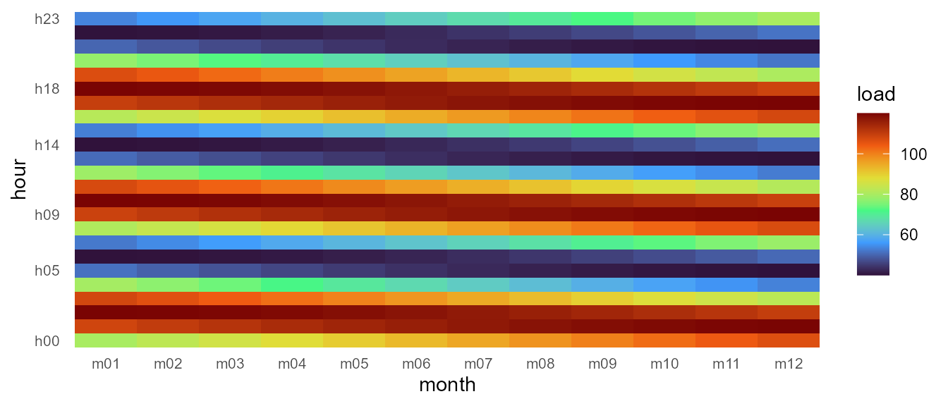
Where to next?
- Concepts — the core ideas behind calendars and timeframes.
-
Data structures — anatomy of a
Calendarobject and its supporting registries. - Data manipulation — the tidy workflow end to end: attach, recast, crosswalks, backends.
- Calendars — the built-in catalog, fiscal years, and wall calendars.
- Visualization — the ggplot2 integration contract and the full plot-type tour on real weather data.