Plot a calendar

One function for every calendar figure, selected by type: the structure icicle (default), the axonometric stack, a heatmap of data on a timeframe grid, and a wall calendar. autoplot() on a Calendar returns the same ggplot; plot() draws it and returns it invisibly.

Usage

gg_calendar(
  object,
  type = c("icicle", "stack", "heatmap", "wall"),
  data = NULL,
  z = NULL,
  key = NULL,
  year = NULL,
  rule = "weighted_mean",
  by = "hour",
  fun = mean,
  palette = NULL,
  labels = NULL,
  reference = NULL,
  annual = TRUE,
  fill = c("order", "share", "weight"),
  color_pattern = c("within", "global"),
  max_labels = 60L,
  max_segments = 2000L,
  border = NA,
  view = NULL,
  angle = NULL,
  ratio = NULL,
  shear = 0.5,
  depth = 0.3,
  gap = NULL,
  rotate = 0,
  direction = c("up", "down"),
  colour = "grey35",
  linewidth = 0.2,
  frame = NULL,
  frame_fill = NA,
  connectors = FALSE,
  x_tf = NULL,
  y_tf = NULL,
  facet_tf = NULL,
  arrange = c("weekday", "sequence"),
  week_start = "MON",
  ...
)

# S3 method for class 'Calendar'
autoplot(object, ...)

# S3 method for class 'Calendar'
plot(x, ...)

Arguments

object: A Calendar.
type: The figure: "icicle" (default), "stack", "heatmap" or "wall"; see the sections below. An argument that belongs to another type is an error, not ignored.
data, z: Colour the figure by a value instead of by structure. data is a data.frame keyed by timeslice (see key) with the value column named by z; z is required whenever data is given. The icicle and the stack recast the value to every timeframe shown, so the whole figure shares one continuous fill scale; the heatmap and the wall collapse the leaves into the cells shown with fun. Legend title via labs(fill = ).
key: Key column of data. NULL (default) uses timeslice when present; the wall also accepts a POSIXct/Date column and detects the first one.
year: The calendar year the figure is about: the wall arranges its days by that year's weekdays, the icicle and the stack route their recasts through it (required with data, see recast_calendar()).
rule, fun: Aggregation. rule is the registry rule of the per-timeframe recasts on the icicle and the stack ("sum", "mean", "weighted_mean", ... as in recast_calendar(); explicit or registered, never guessed). "share" colours every row by each timeslice's share within the row above it on a fixed linear 0..1 scale; "logshare" is the same on a fixed log10 percent scale. fun is the function that collapses several observations into one cell on the heatmap and the wall (default mean).
by: With data on the icicle or the stack: base-grid granularity of the recasts. Defaults to "hour", which is always correct (the automatic choice can pick a daily grid for sub-daily calendars, which silently collapses hour-type slices).
palette: Fill scale. NULL (default) is the type's own: viridis "D" on the icicle and the stack, ggplot2's default gradient on the heatmap and the wall. A viridis option letter or name ("C", "plasma", "turbo", ...) opts into that palette on any type. NA adds no fill scale at all, so a custom one can be supplied.
labels: What is labelled. NULL (default) is the type's own. Icicle: "name" (the member value, e.g. h00; the default), "timeslice" (the full path, e.g. Q1_h00) or "none"; TRUE and FALSE are shorthands. Stack: a character vector of timeframes whose member names are drawn on their plane (TRUE = all; default none). Wall: TRUE (default) draws the day numbers. The heatmap has no labels.
reference: Icicle only: a complete Calendar to draw a sampled object against. The layout is the reference's; segments without a timeslice of object are left empty (grey). TRUE resolves the reference from meta$parent_name, as recorded by filter_calendar().
annual: Icicle and stack: include the ANNUAL root. Default TRUE.
fill: Icicle: what drives the structure fill, "order" (chronological position, default), "share" or "weight". data overrides it.
color_pattern: Icicle, for fill = "order": "within" (default) restarts the gradient inside each parent timeslice (hours recycle every day); "global" sweeps once across the whole year.
max_labels: Icicle: rows with more segments than this get no labels. Default 60.
max_segments: Icicle: rows with more segments than this are binned by x-midpoint before drawing (fill = width-weighted mean), keeping hourly calendars fast. Default 2000.
border: Icicle: rectangle border colour. Default NA (none), so dense rows render as smooth gradients.
view: Stack: a predefined point of view – "oblique" (the shear/depth default), "top-down", "cavalier", "cabinet", "military", "isometric", "dimetric", "trimetric", "perspective" (receding planes shrink) or "pyramid" (receding planes grow: the coarsest timeframe is the small top, the finest the wide base).
angle, ratio: Stack: oblique view by angle (degrees of the receding axis) and foreshortening ratio – e2 = ratio * (cos(angle), sin(angle)). Overridden by view.
shear, depth, gap: Stack: the raw receding-axis components (e2 = (shear, depth); used when neither view nor angle/ratio is given) and the vertical spacing between planes: one value for every pair, or one per pair from the top down. gap = NULL (default) spaces planes almost touching, with a slight overlap (0.85 x the plane's screen height). Under "perspective" and "pyramid" each spacing is scaled with the planes it separates, so it stays uniform relative to their size.
rotate: Stack: in-plane rotation of each plane (degrees, counter-clockwise) before projection.
direction: Stack: "up" (default) stacks the coarsest timeframe on top; "down" puts it at the bottom.
colour, linewidth: Stack: segment border colour and width, recycled across the planes (one entry per plane styles them individually). Defaults "grey35" and 0.2, ggplot2's own sf polygon border. The icicle's rectangle border is the separate border argument.
frame: Stack: draw each plane's outline (the unit box run through the same projection) as a guide. TRUE uses "grey80", a colour string uses that colour, NULL (default) draws no frames.
frame_fill: Stack: fill for the plane sheets; best mostly transparent, e.g. frame_fill = ggplot2::alpha("grey60", 0.12). Setting a fill draws the frames even without frame; NA (default) = no fill.
connectors: Stack: dashed lines joining the corresponding frame corners of adjacent planes. TRUE uses the frame colour, a colour string picks its own; default FALSE.
x_tf, y_tf, facet_tf: Heatmap: timeframe names overriding the automatic layout (finest timeframe on y, next-finest on x, anything coarser as facets).
arrange: Wall: "weekday" (default) places each day under its weekday of year; "sequence" fills the week grid in order.
week_start: Wall: first day of the week. Default "MON".
...: Fixed aesthetics for the figure's main layer: the icicle's geom_rect(), the stack's plane polygons, the heatmap's and the wall's geom_tile() (e.g. alpha = 0.8).
x: A Calendar (for plot()).

Value

A ggplot object.

Icicle (`type = "icicle"`)

One horizontal band per timeframe (ANNUAL root on top, coarsest first), rectangle widths proportional to timeslice shares, x spanning the covered year on [0, 1]. With data, each band's rectangles carry the value recast to that band's timeframe; dense bands are binned with width-weighted means.

Stack (`type = "stack"`)

The same structure drawn axonometrically: one sheared plane per timeframe, ANNUAL on top, each plane segmented by the true duration shares, with segments visibly nesting into the plane above. Without data, each plane is coloured by its own segment order.

Heatmap (`type = "heatmap"`)

Data on a timeframe grid: finest timeframe on y, next-finest on x, anything coarser as facets (overridable via x_tf/y_tf/facet_tf). Without data, the calendar's own share is drawn.

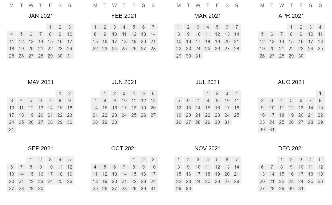
Wall (`type = "wall"`)

A wall calendar: one facet per month (in member order, so April first for the fy04_* fiscal calendars), day cells in a week grid, weeks top-down. data may be keyed by timeslice (day-level ids directly; finer ids, e.g. hours of d365_h24, roll up into their day cell) or by datetime (mapped through datetime_to_timeslice() on the day layer). Needs a day-resolution timeframe (YDAY or MDAY).

Methods

autoplot(object, ...) is gg_calendar(object, ...). plot(x, ...) prints that figure and returns it invisibly, like base plot().

Examples

if (requireNamespace("ggplot2", quietly = TRUE)) {
  cal <- calendar("q4_h24")
  gg_calendar(cal)
  ggplot2::autoplot(cal)                            # the same figure
  gg_calendar(calendar("s4_hp3"), type = "stack")

  x <- data.frame(timeslice = sprintf("m%02d", 1:12), load = 1:12)
  gg_calendar(calendar("m12"), data = x, z = "load", type = "heatmap")

  gg_calendar(calendar("m12_md365"), type = "wall", year = 2021)
}

Usage

Arguments

Value

Icicle (type = "icicle")

Stack (type = "stack")