Plotting geoscales

library(geoscales)

A map to draw on

geoscales ships no map data, so this article borrows one. The UTOPIA reference regions from energyRt are ideal for it: eleven regions nested nation -> zone -> region, entirely offline, and completely invented — so nothing here depends on a network, a licence, or any real-world boundary.

gs <- energyRt::utopia_geoscale("honeycomb")
gs
#> Geoscale: utopia 
#> Description: UTOPIA reference regions, nested nation -> zone -> region 
#> Levels (3, coarsest first):
#>   - nation (1)
#>     - zone (3)
#>       - region (11)
#> Atoms: 11
#> Weights: area (default: area)
#> CRS: NA
#> Geometry: attached (11 features)

That one call returns a finished Geoscale: hierarchy, geometry and an area weight. Everything from here on is plain geoscales.

head(as.data.frame(S7::prop(gs, "leaves")), 4)
#>   nation    zone region     name     area
#> 1 UTOPIA    WEST     R1 Oswestia 5.655895
#> 2 UTOPIA    WEST     R2  Antidia 5.655895
#> 3 UTOPIA    WEST     R3  Kopalia 5.655895
#> 4 UTOPIA CENTRAL     R4   Kalgia 5.655895

Two views of the same object

A Geoscale is a hierarchy that may carry geometry, and the two are drawn by different functions. geo_autoplot() shows the structure — one row per level, widths proportional to weight — and needs no geometry at all:

geo_autoplot(gs)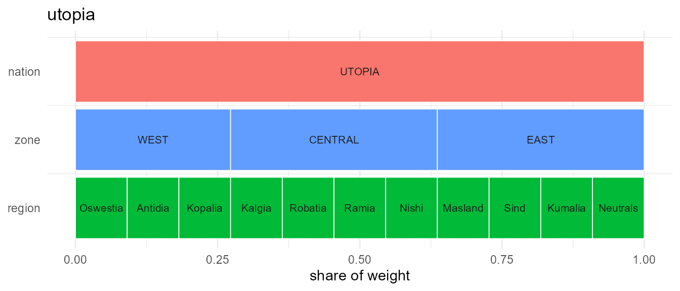

geo_plot() shows the same regions in space:

geo_plot(gs, label = TRUE)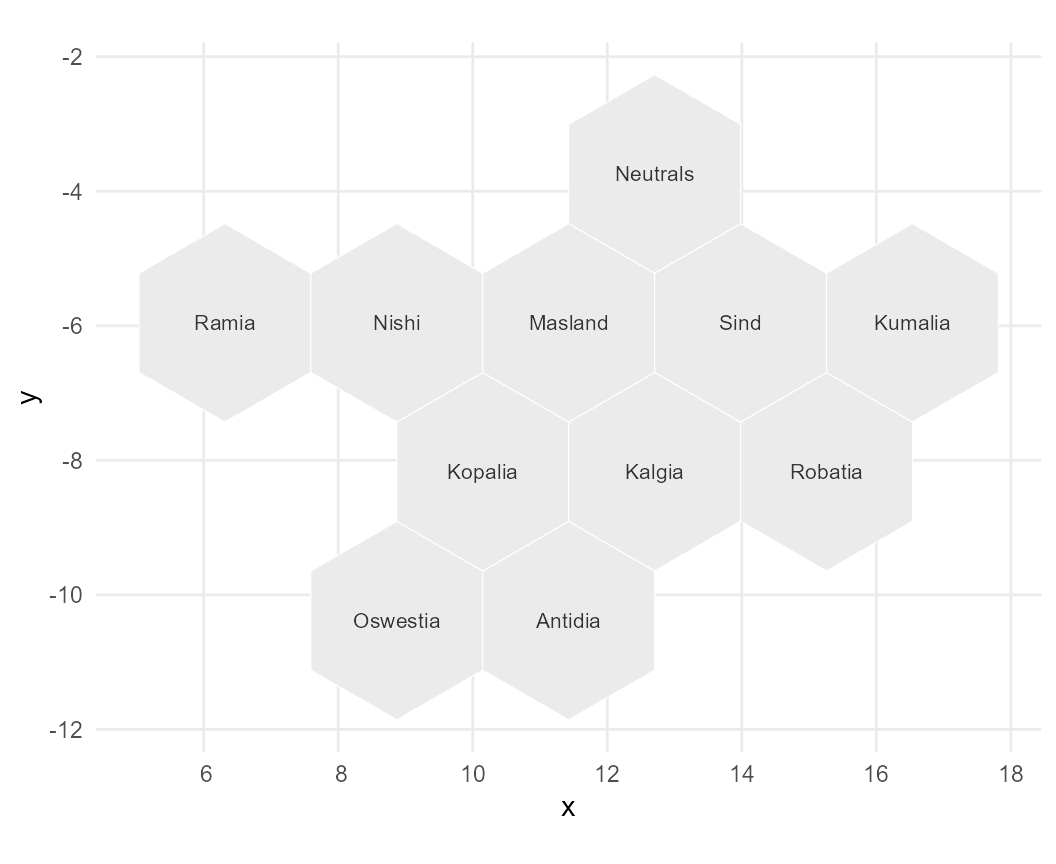

Note the labels. The icicle above says WEST, CENTRAL, EAST but the map says Oswestia, Antidia, …: a geoscale can declare a column of display names (labels = "name" here), and they are used wherever they are unambiguous. A zone made of Oswestia and Antidia has no name of its own, so it keeps its code rather than borrowing one of its parts.

Geometry is separable from hierarchy

UTOPIA ships four alternative layouts. The hierarchy is identical in all of them — only the shapes differ, which is exactly the point: a Geoscale is a nesting first and a map second.

geo_geometry() returns an ordinary sf object, so combining the layouts into one faceted figure needs nothing from this package:

layouts <- c("squares", "honeycomb", "island", "continent")

shapes <- do.call(rbind, lapply(layouts, function(l) {
  s <- geo_geometry(energyRt::utopia_geoscale(l), level = "region")
  s$layout <- l
  s
}))

ggplot2::ggplot(shapes) +
  ggplot2::geom_sf(fill = "grey92", colour = "white") +
  ggplot2::facet_wrap(~layout) +
  ggplot2::theme_minimal()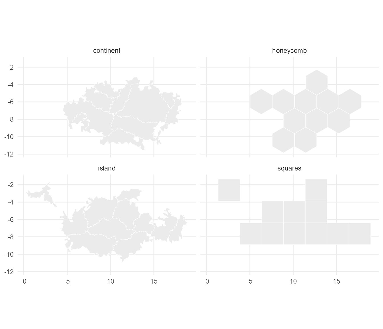

One level per panel

geo_plot(level = ) dissolves the atoms up to whichever level you ask for. Eleven regions become three zones become one nation:

levels_sf <- do.call(rbind, lapply(geo_levels(gs), function(l) {
  s <- geo_geometry(gs, level = l)
  names(s)[1] <- "code"
  s$level <- l
  s
}))
levels_sf$level <- factor(levels_sf$level, levels = geo_levels(gs))

ggplot2::ggplot(levels_sf) +
  ggplot2::geom_sf(ggplot2::aes(fill = code), colour = "white",
                   show.legend = FALSE) +
  ggplot2::facet_wrap(~level) +
  ggplot2::theme_minimal()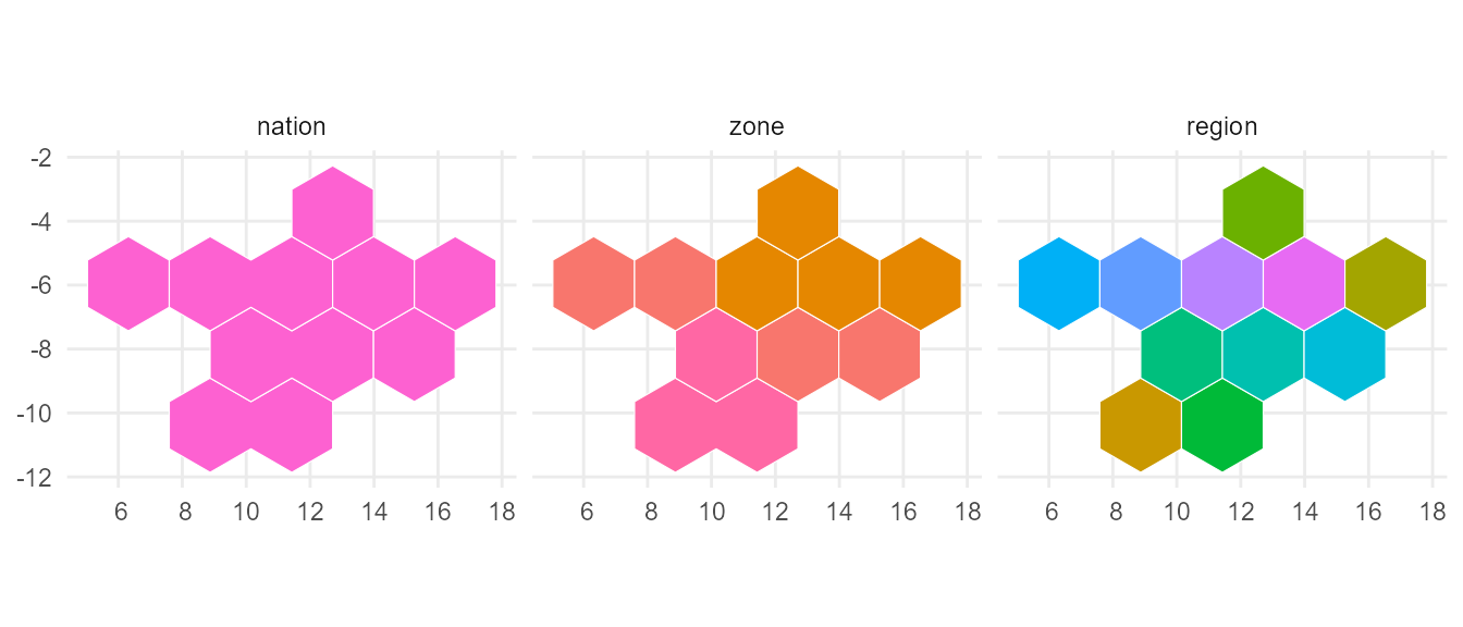

Values on the map

Pass a data.frame with a column named after the level, and name the column to colour by:

set.seed(1)
gen <- data.frame(region = geo_regions(gs, "region"),
                  gen = round(runif(11, 10, 100)))

geo_plot(gs, gen, level = "region", fill = "gen",
         palette = "D", title = "Generation", subtitle = "TWh by region")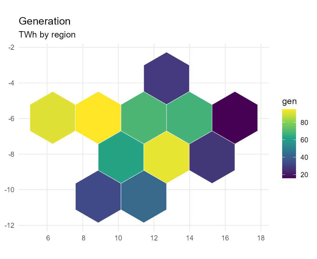

geo_plot() is the package’s only choropleth renderer, and it is deliberately ignorant of what your numbers mean. Callers that do know — energyRt::geo_map() is one — prepare the data.frame and hand it here rather than drawing their own geom_sf().

Recasting, seen on the map

geo_recast() is the one verb that moves data between levels, in both directions. Aggregating eleven regions into three zones with rule = "sum":

by_zone <- geo_recast(gen, gs, from = "region", to = "zone", rule = "sum")
by_zone
#>      zone gen
#> 1 CENTRAL 306
#> 2    EAST 181
#> 3    WEST 139
sum(by_zone$gen) == sum(gen$gen)
#> [1] TRUE

geo_plot(gs, by_zone, level = "zone", fill = "gen",
         palette = "D", title = "Generation", subtitle = "aggregated to zones",
         label = TRUE)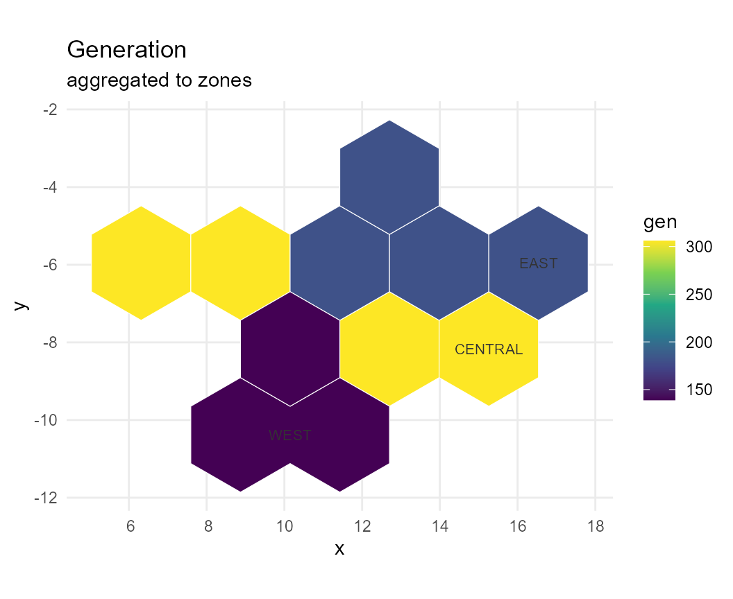

The same verb runs back down. Going down, rule = "sum" splits each total in proportion to a weight, so the national figure is conserved:

national <- data.frame(nation = "UTOPIA", gen = 1000)
split_back <- geo_recast(national, gs, from = "nation", to = "region",
                         rule = "sum", weight = "area")

geo_plot(gs, split_back, level = "region", fill = "gen", palette = "D",
         title = "A national total split by area")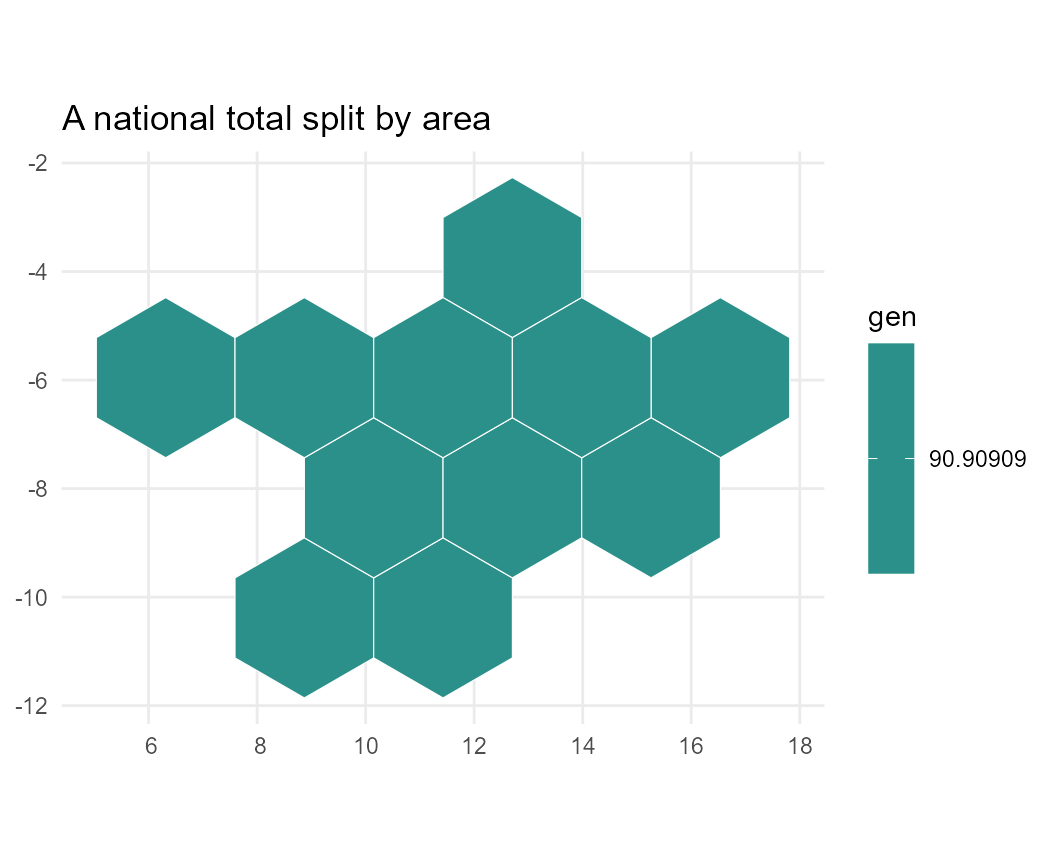

Extensive and intensive quantities

The rule matters, and the map makes the difference obvious. Generation adds up — it is extensive, so sum is right. A capacity factor does not: averaging it needs a weight, and summing it is meaningless.

cf <- data.frame(region = geo_regions(gs, "region"),
                 cf = round(runif(11, 0.2, 0.6), 2))

right <- geo_recast(cf, gs, "region", "zone", rule = "weighted_mean",
                    weight = "area")
wrong <- geo_recast(cf, gs, "region", "zone", rule = "sum")
merge(right, wrong, by = "zone", suffixes = c("_weighted_mean", "_sum"))
#>      zone cf_weighted_mean cf_sum
#> 1 CENTRAL        0.5000000   2.00
#> 2    EAST        0.4275000   1.71
#> 3    WEST        0.3633333   1.09

Every value in the sum column is above 1.0, and a capacity factor above 1.0 is not a number that exists. The weighted mean stays in range because it asks how much of each region there is; the sum does not. Register the rule once per parameter and it cannot be got wrong twice — see vignette("geoscales").

Subsetting

geo_filter() returns a smaller Geoscale, geometry included, so it plots like any other:

west <- geo_filter(gs, level = "zone", region = "WEST")
geo_plot(west, label = TRUE, title = "WEST only")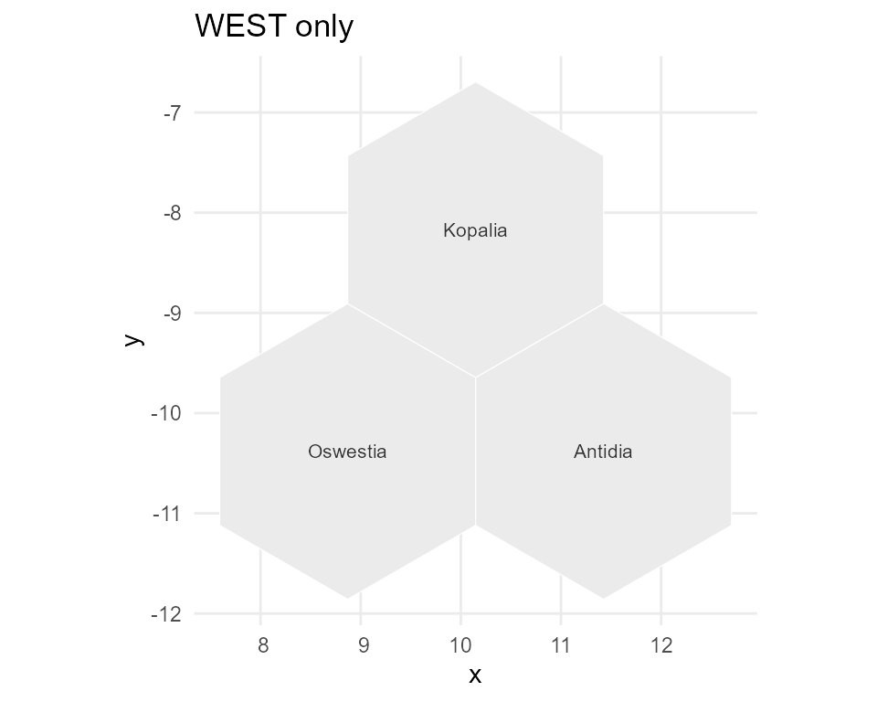

Bringing your own source

UTOPIA arrived here as a plain function call, but any source can be registered with the provider interface that rnaturalearth uses — see vignette("from-naturalearth"):

geo_register_provider(
  "utopia",
  fetch = function(layout = "honeycomb") {
    merge(energyRt::utopia$geo, energyRt::utopia$map[[layout]], by = "region")
  },
  levels = c("nation", "zone", "region"),
  desc = "UTOPIA reference regions (energyRt)"
)
geoscale_from_provider("utopia")