Calendar layers for ggplot2 — geom

Composable single layers that put time-series data on a calendar inside a normal ggplot() pipeline (the assembled-figure counterparts are calendar_autoplot() and calendar_plot()):

Usage

geom_calendar(
  calendar,
  z,
  datetime = "datetime",
  by = NULL,
  x_tf = NULL,
  y_tf = NULL,
  fun = mean,
  data = NULL,
  ...
)

geom_calendar_tile(
  calendar,
  z,
  timeslice = "timeslice",
  by = NULL,
  x_tf = NULL,
  y_tf = NULL,
  fun = mean,
  data = NULL,
  ...
)

theme_calendar(...)

Arguments

calendar: A Calendar.
z: Name of the numeric column to aggregate and fill by.
datetime: Name of the POSIXct/Date column (geom_calendar()). Default "datetime".
by: Character vector of columns to preserve through aggregation (facet/group carriers). Default none.
x_tf, y_tf: Timeframes for the x and y axes. Default: finest on y, next-finest on x.
fun: Aggregator over instants/timeslices falling in one tile. Default mean.
data: A data.frame; NULL (default) uses the plot data.
...: Passed to the tile geom (e.g. colour, linewidth), or for theme_calendar() to ggplot2::theme().
timeslice: Name of the timeslice-ID column (geom_calendar_tile()). Default "timeslice".

Value

A single ggplot2 layer (theme_calendar() returns a theme).

Details

geom_calendar() — datetime mode: name a POSIXct/Date column (datetime=) and a measured column (z=); instants are cut to timeslices via datetime_to_timeslice() and aggregated with fun.
geom_calendar_tile() — timeslice mode: name a timeslice-ID column (timeslice=) and the measured column (z=).
theme_calendar() — the compact heatmap theme the assembled plots use.

The calendar inputs are column names, not aes() mappings: ggplot2 trains positional scales before statistics run, so a ggproto Stat cannot emit the discrete axes a calendar heatmap needs. Each function instead returns one standard tile layer whose data is derived from the plot (or layer) data — discrete scales, facets, and themes then work through the normal ggplot2 path. The tile fill is the aggregated value; axes are vocabulary-ordered factors, so scale_x_discrete() etc. apply as usual.

Faceting: list the columns your facets need in by= — aggregation then happens within each combination and the columns survive into the layer data (see the example).

Examples

if (requireNamespace("ggplot2", quietly = TRUE)) {
  library(ggplot2)
  cal <- calendar("m12_h24")

  # datetime mode with a facet carrier
  x <- data.frame(
    t = as.POSIXct("2021-01-01", tz = "UTC") + 3600 * (0:999),
    v = rnorm(1000),
    site = rep(c("A", "B"), 500)
  )
  ggplot(x) +
    geom_calendar(calendar = cal, datetime = "t", z = "v", by = "site") +
    facet_wrap(~site) +
    theme_calendar()

  # timeslice mode
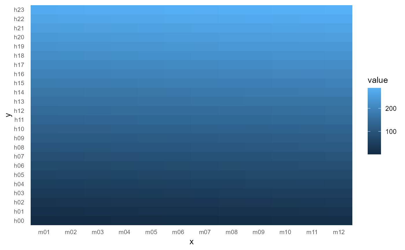
  y <- data.frame(timeslice = S7::prop(cal, "leaftable")$timeslice, v = 1:288)
  ggplot(y) +
    geom_calendar_tile(calendar = cal, z = "v") +
    theme_calendar()
}