Wall-calendar figure

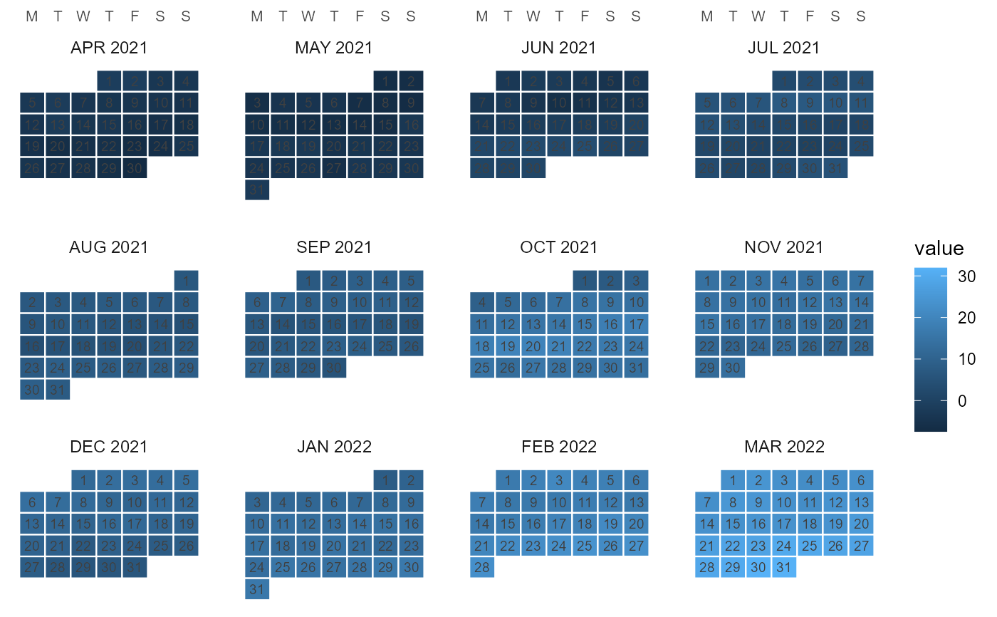
Draws the calendar as a wall calendar: one facet per month (in member order – April first for the fy04_* fiscal calendars), day cells in a week grid, weeks top-down. With data, day cells are filled by the aggregated value; without, a plain calendar (day numbers only).

Usage

calendar_wall_plot(
  x,
  data = NULL,
  z = NULL,
  year = NULL,
  arrange = c("weekday", "sequence"),
  week_start = "MON",
  fun = mean,
  label = TRUE,
  key = NULL,
  ...
)

Arguments

x

A Calendar with a day-resolution timeframe (YDAY or MDAY). Sub-daily timeframes are collapsed to the day layer via prune_calendar().

data

Optional data.frame of values to fill the day cells.

z

Name of the numeric value column of data.

year

Integer model year (required for the weekday arrangement; NULL falls back to "sequence" with a message).

arrange

"weekday" or "sequence" (see above).

week_start

Weekday the week starts on: one of "MON".."SUN" (default "MON", ISO).

fun

Aggregator collapsing multiple observations (sub-daily timeslices, repeated dates) into one day cell. Default mean.

label

Draw day-of-month numbers (default TRUE).

key

Key column of data; NULL auto-detects.

...

Passed to ggplot2::theme() via theme_calendar().

Value

A ggplot object.

Details

data may be keyed by timeslice (day-level IDs directly; finer IDs – e.g. hours of d365_h24 – roll up into their day cell) or by datetime (mapped through datetime_to_timeslice() on the day layer). The key column is auto-detected (timeslice, else the first POSIXct/Date column) unless key= names it.

Examples

if (requireNamespace("ggplot2", quietly = TRUE)) {
  # plain wall calendar for 2021
  calendar_wall_plot(calendar("m12_md365"), year = 2021)

  # daily data on a fiscal wall (April..March facets)
  cal <- calendar("fy04_d365")
  x <- data.frame(
    timeslice = S7::prop(cal, "leaftable")$timeslice,
    v = cumsum(stats::rnorm(365))
  )
  calendar_wall_plot(cal, x, z = "v", year = 2021)
}