Data sources

library(reneuro)
library(dplyr)

The 41-node data page shows the processed data as it enters the model. This article is everything upstream of that: the raw sources, how the renewable potentials and profiles are made, and the NUTS-level datasets (nuts_gs, nuts_load, nuts_lines) with the aggregation arithmetic that turns them into any coarser regional layer. The heavy inputs (a 6.7 GB weather cutout, a PyPSA-Eur clone) do not ship, so their figures are pre-rendered by data-raw/data_sources_figures.R and data-raw/cf-workflow/ and committed; everything drawn from shipped data is computed live on this page.

1. Weather: the cutout

Wind and solar availability come from one file: the cutout europe-2025-sarah3-era5.nc — a 0.3° grid over Europe (177 × 131 cells) with 8,760 hourly fields of wind speed, solar irradiance, temperature and runoff for 2025. This is raw meteorology, not capacity factors: 100 m wind speed (ERA5, regridded from its native 0.25°), direct and diffuse solar influx (SARAH-3 satellite data, aggregated from its native 0.05° and 30-minute resolution). A 0.3° cell is roughly 21 × 33 km at European latitudes. PyPSA-Eur turns it into per-region hourly capacity factors; those arrive in the models as the weather objects (W_ONWIND, W_SOLAR, …).

These are one weather year. The horizon series reuses the same profiles to 2050, so 2025 sets both the variability and the potential throughout. The wind and solar articles take the potential from long-term atlases instead, keeping these hours for the variability.

fig("cutout-wind.png")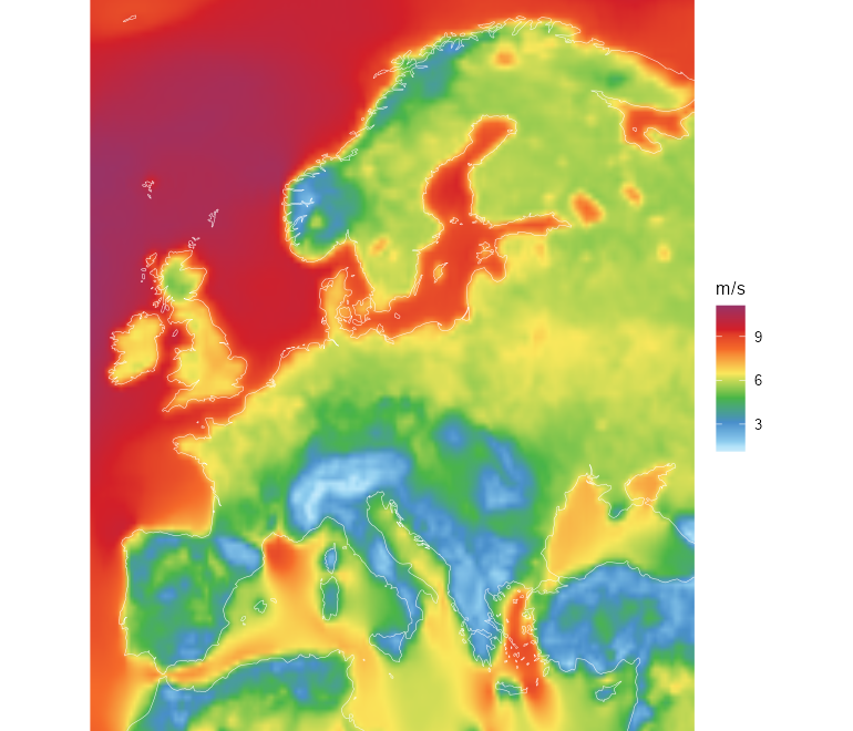

Mean 100 m wind speed over 2025, from the ERA5 fields of the cutout (CC-BY, Copernicus Climate Change Service).

fig("cutout-solar.png")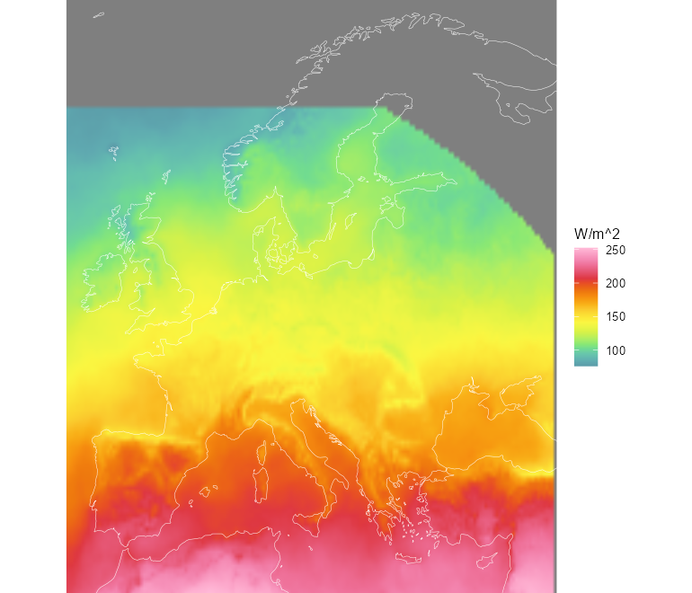

Mean solar influx (direct + diffuse) over 2025 — the SARAH-3 satellite record (CC-BY, EUMETSAT CM SAF) with ERA5 infill at high latitudes.

The exact licence notices ship in system.file("LICENSE.note", package = "reneuro").

A second, much finer wind source complements the cutout: the Global Wind Atlas at 250 m, carved into capacity-factor bands for the quality-aware resource layer (see the wind article). Where the cutout gives one number per ~25 km cell, the atlas resolves individual ridgelines and coastal gradients:

fig("gwa_carved_map.png", "cf-pipeline")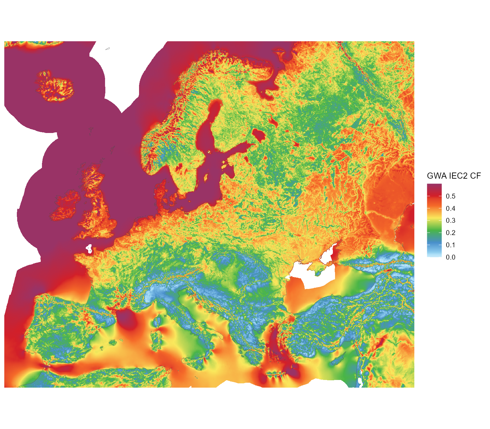

Global Wind Atlas IEC2 capacity factor at 250 m; land and sea shown, the land-eligibility screen applies downstream.

2. Demand: measured ENTSO-E series

Hourly national load for 2025 comes from the ENTSO-E transparency platform (with NESO for Great Britain). It lands in the models as each region’s demand, distributed below country level by a GDP/population proxy.

fig("demand-entsoe.png")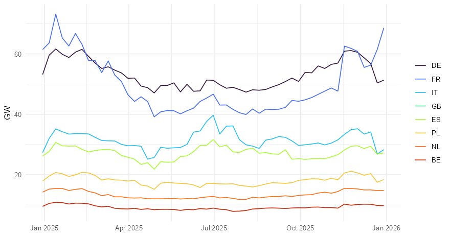

Weekly-mean measured demand for the eight largest systems, ENTSO-E transparency platform. The workflow fills the few countries with gaps (UA, MK, CY, AL) from template years.

The 2025 total across the modelled countries is 3,163 TWh — visible in the shipped models as the sum over the demand objects:

objs <- pypsa_eur_41@data[[1]]@data
dem <- objs[vapply(objs, function(o) class(o)[1], "") == "demand"]
sum(vapply(dem, function(d) sum(d@demand$demand), 0)) / 1e6  # TWh
#> [1] 3162.754

3. The existing fleet

Power plants come from powerplantmatching, which deduplicates GEM, JRC, ENTSO-E, GPD and other registries into one unit list — 157,549 units with coordinates and capacities. In the models they become the non-extendable stock (nuclear, coal, hydro, …) and the cap.lo floors on extendable carriers (wind, solar); in the pypsa_eur_41_<year> horizon series they also drive retirement, through announced closure dates where they exist and assumed lifetimes elsewhere.

fig("fleet.png")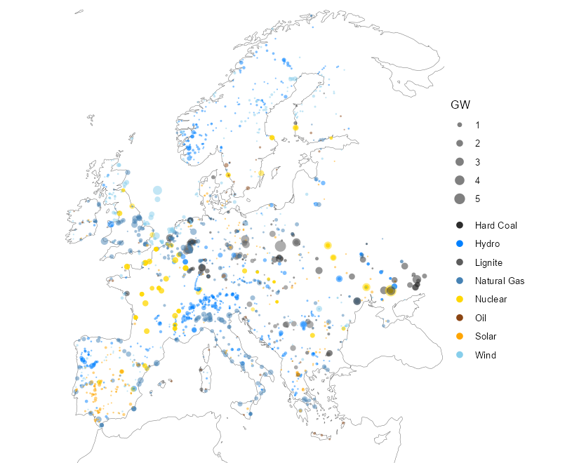

The existing fleet: units of 100 MW and above, sized by capacity, coloured by fuel — powerplantmatching (GEM, JRC, ENTSO-E, GPD and more, deduplicated).

4. The network source

Transmission comes from OpenStreetMap (which is what makes the shipped data ODbL): substations and lines, simplified and clustered by PyPSA-Eur. In the models it is the trade corridors — drawn on the 41-node data page; the NUTS-level line dataset and its aggregation arithmetic are documented below.

5. How potentials and profiles are made

Every wind and solar generator in the shipped models traces back to two PyPSA-Eur artifacts: a potential (p_nom_max, the MW that may be built per region) and a profile (p_max_pu, the hourly capacity factor). The order of the pipeline matters more than any single step: clustering comes first. PyPSA-Eur clusters a network that contains no generators at all, and only then computes land eligibility, potentials, and profiles directly on the clustered regions — the blending happens once, from weather cells straight into whatever region set was chosen.

1. Weather cutout — the single 0.3° grid above.
2. Land eligibility — per carrier, a 100 m exclusion mask built from CORINE land cover, Natura 2000 protected areas, a 1 km urban buffer (onshore wind), ship density, water depth and shore distance (offshore). The eligible share of each 0.3° cell within each region becomes the availability matrix. No criterion involves the resource itself — no wind speed, no irradiation, no slope, no altitude.
3. Potential — p_nom_max = eligible area × a flat deployment density (3 MW/km² onshore wind, 5.1 solar, 2 offshore). Every eligible km² counts the same, whatever its wind.
4. Profile — capacity factors are computed per cell from the cutout (Vestas V112 3 MW power curve onshore; crystalline-silicon panel at 35° tilt), then blended into one regional series with weights proportional to each cell’s mean capacity factor — “more generators are installed at better sites”.

Two properties follow that most users don’t expect:

The asymmetry. The potential counts all eligible land, but the profile is weighted toward the best cells. A region therefore offers its entire eligible area at close to its best-sites capacity factor — an optimistic bias that grows with region size and internal resource spread. At 41 nodes regions span whole countries; at NUTS3 the bias is mildest.

Nothing is filtered by quality. Regions whose mean wind capacity factor is 0.2% survive alongside ones at 54%; a 0.094 MW potential is carried through. A binning mechanism exists upstream (resource_classes) that would split each region into capacity-factor tiers, but it is off by default and off in these builds — each region gets exactly one blended generator per carrier.

The quality-aware alternative built beside the original is documented in the wind and solar potential articles.

6. The land itself

The CORINE raster behind the exclusions, at CLC level 1, and what the per-carrier grid-code inclusion admits from it. Wind’s base is agriculture plus forest and natural land; solar trades the forests for artificial surfaces. About half the wind-only area is forest.

fig("corine_landtype.png", "cf-pipeline")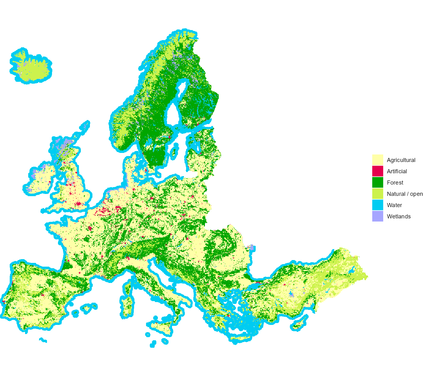

CORINE land cover at CLC level 1 (~5 km modal aggregate of the 250 m raster).

fig("corine_eligibility.png", "cf-pipeline")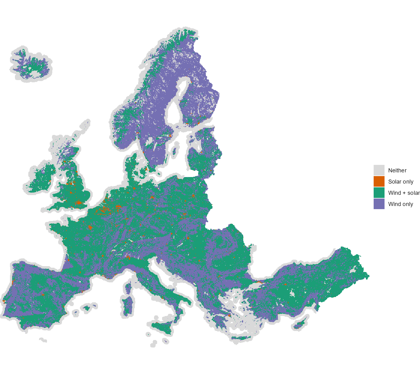

Land admitted by the PyPSA-Eur CORINE grid-code coding, per carrier. Inclusion only — Natura 2000, urban buffers and the other excluders apply on top.

7. Available land

The availability matrices behind the shipped models, drawn at the cutout’s own resolution. Dark cells are excluded (urban fabric and its buffer for wind, forests for solar, protected areas for both); the eligible remainder is dominated by agricultural land, which no exclusion touches.

fig("avail_map_onwind.png", "cf-pipeline")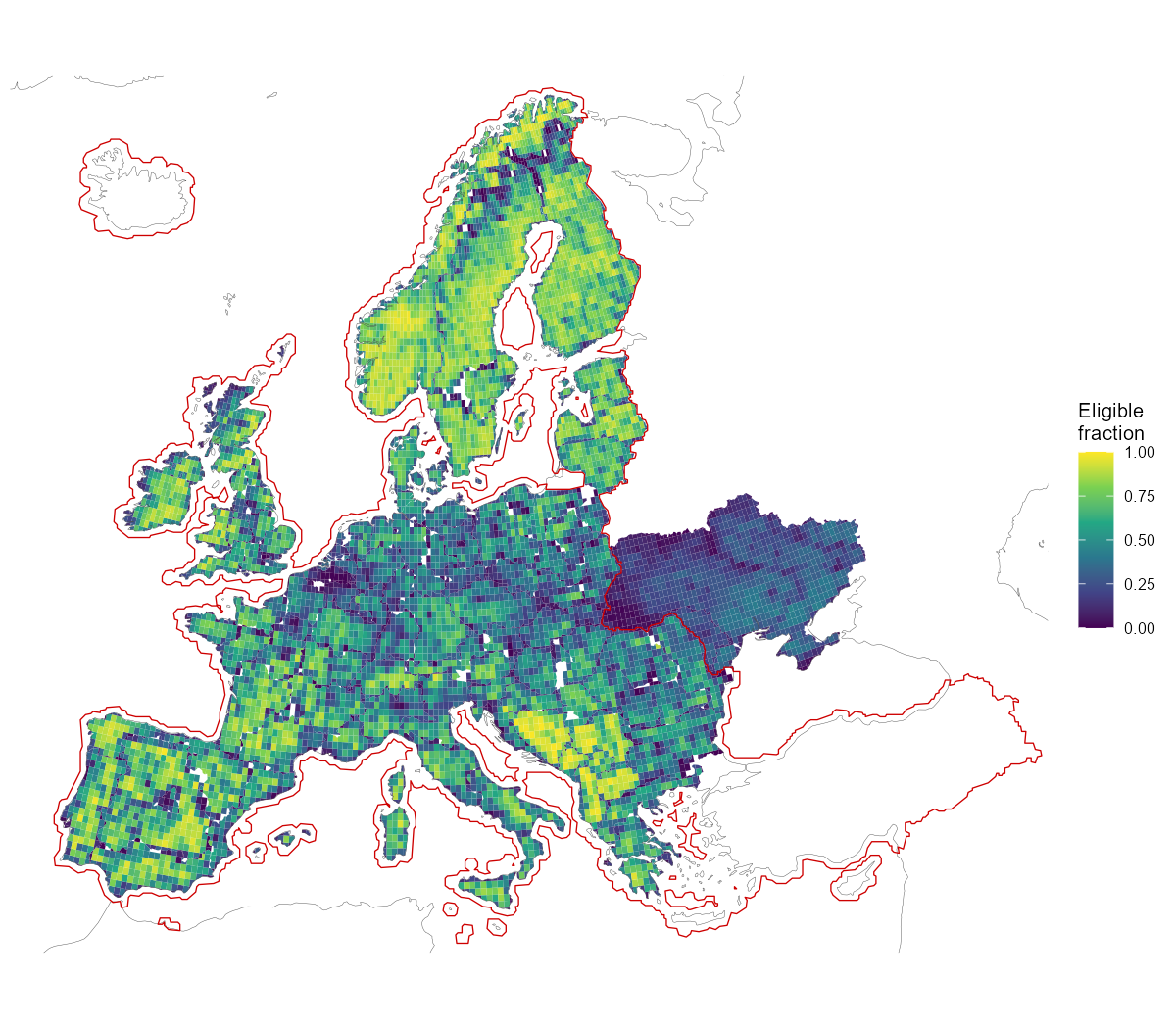

Available land for onshore wind: eligible share of each region-clipped cell after the land-use exclusions. The solid red line traces the CORINE raster coverage; outside it the shown fraction carries the flat 0.5 derate.

fig("mwmax_map_onwind.png", "cf-pipeline")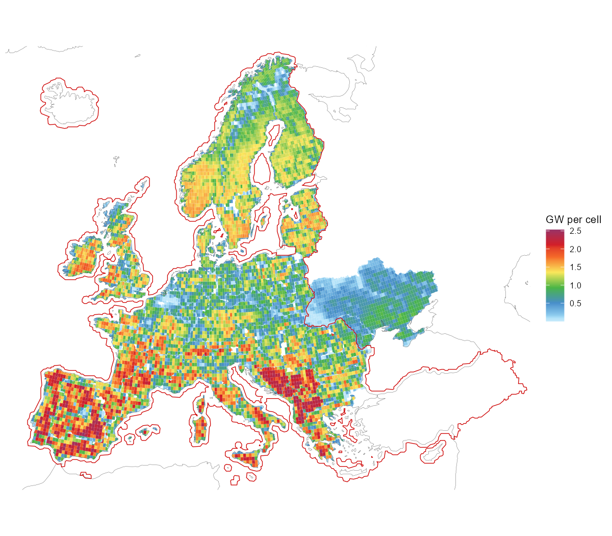

Installable onshore wind potential per cell: eligible area × 3 MW/km² (unfiltered; flat 0.5 derate outside the red CORINE coverage line).

Reconciliation: eligible area × density reproduces PyPSA’s p_nom_max exactly (to the megawatt) for wind and all offshore carriers. Solar differs by +1.8%, and the entire difference sits in cells north of 65°N: SARAH-3 has no data there, and PyPSA silently drops that eligible land from the solar potential rather than excluding it by policy.

8. The NUTS datasets

Three shipped datasets carry the regional layer the models are built on: nuts_gs (the geography and the data attached to it), nuts_load (demand) and nuts_lines (transmission). Each section below aggregates one of them from NUTS3 to coarser levels and gives the arithmetic used, which differs by quantity: capacities sum, per-capita values take a weighted mean, and peaks and impedances have to be recomputed rather than combined.

Nested levels

gs <- nuts_gs
vapply(geoscales::geoscale_geoframes(gs),
       function(f) length(geoscales::geoscale_regions(gs, f)), 0L)
#> europe  nuts0  nuts1  nuts2  nuts3 
#>      1     36    109    296   1477

1,477 NUTS3 atoms group into 296 NUTS2, 109 NUTS1, 36 countries and a single europe root. Every finer code has exactly one parent; the build asserts this rather than assuming it, and the aggregation below depends on it.

The europe root is the only region at which a continental commodity balance can be declared. newCommodity(geoframe = "europe") gives one Europe-wide CO2 allowance or gas market; without it the coarsest balance is per country, i.e. 36 separate markets.

library(geoscales)

lt <- as.data.frame(geoscale_leaftable(nuts_gs))

geoscale_autoplot(nuts_gs, type = "stack", direction = "down",
                  view = "oblique", colour = NA,
                  frame = T, frame_fill = ggplot2::alpha("grey60", 0.12),
                  data = lt, z = "cap_mw", rule = "share")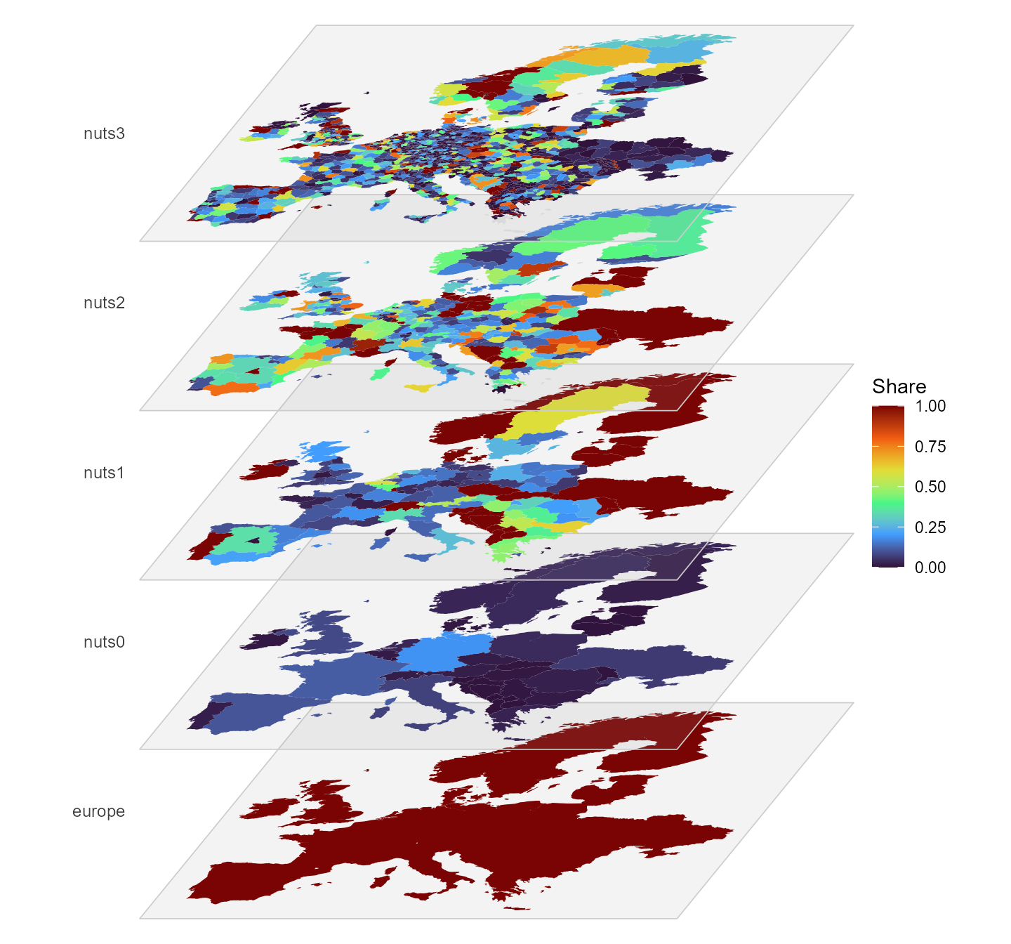

The region hierarchy as a multilayer stack, each plane one level, coloured by each region’s share of its parent’s existing generation capacity (cap_mw).

The same hierarchy as an icicle plot. The NUTS3 row is omitted: at 1,477 atoms most rectangles are thinner than their own outline, so the level reads as a solid band and adds nothing:

gs2 <- geoscales::geoscale_from_leaftable(
  lt |> summarise(km2 = sum(km2), .by = c(europe, nuts0, nuts1, nuts2)),
  geoframes = c("europe", "nuts0", "nuts1", "nuts2"),
  key = "nuts2", weights = "km2")
energyRt::plot_geoscale(gs2, type = "icicle")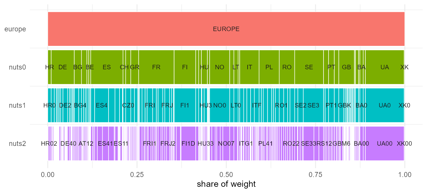

The region hierarchy as an icicle, europe down to NUTS2; widths are area shares.

Four countries — BA, MD, UA, XK — have no NUTS at all and are filled from OpenStreetMap adm1. Those regions become the atoms, and the levels above them are padded (MD0, MD00):

lt <- as.data.frame(geoscales::geoscale_leaftable(gs))

# Every aggregation below is "roll the atoms up to a coarser geoframe", which is
# a lookup from the NUTS3 code to its parent at that level. Named once here
# rather than rebuilt inline each time.
parent_of <- function(level, from = "nuts3") setNames(lt[[level]], lt[[from]])

lt |>
  filter(nuts0 %in% c("BA", "MD", "UA", "XK")) |>
  group_by(nuts0) |>
  summarise(atoms = n(), nuts1 = first(nuts1), nuts2 = first(nuts2))
#> # A tibble: 4 × 4
#>   nuts0 atoms nuts1 nuts2
#>   <chr> <int> <chr> <chr>
#> 1 BA        3 BA0   BA00 
#> 2 MD       37 MD0   MD00 
#> 3 UA       27 UA0   UA00 
#> 4 XK        7 XK0   XK00

PyPSA-Eur repeats the adm1 code at every level, which makes each such region its own parent. The derived hierarchy then contains pairs like (MD-BA, MD-BA), and energyRt’s spatial roll-up becomes vOutTot[MD-BA] = ... + vOutTot[MD-BA], forcing every other term to zero without error.

Eurostat’s convention for identical geography is a distinct code per level: Luxembourg is LU → LU0 → LU00 → LU000, and no NUTS country produces an identity pair. The padding here follows that convention. “NUTS1” and “NUTS2” for these four countries remain stand-ins rather than real administrative levels.

f <- geoscales::geoscale_geoframes(gs)
vapply(seq_len(length(f) - 1L),
       function(i) isTRUE(geoscales::geoscale_nests(gs, f[i], f[i + 1L])),
       logical(1))
#> [1] TRUE TRUE TRUE TRUE

Every adjacent pair nests. Where nesting fails, a region has two parents and its balance is added into both.

What each region carries

The leaftable holds 14 data columns per region, in two families. The family determines what a column can be used for.

setdiff(names(lt), c("region", geoscales::geoscale_geoframes(gs)))
#>  [1] "km2"               "pop"               "gdp"              
#>  [4] "gdp_total"         "load_twh"          "peak_mw"          
#>  [7] "n_buses"           "cap_mw"            "hydro_mw"         
#> [10] "pot_onwind"        "pot_solar"         "pot_solar_hsat"   
#> [13] "pot_offwind_ac"    "pot_offwind_dc"    "pot_offwind_float"

Geographic, read from the region shapes and defined for all 1,477 atoms:

column	unit	kind
km2	km², equal-area projection	extensive
pop	thousands	extensive
gdp	EUR per capita	intensive
gdp_total	thousand EUR	extensive

Model, read from the NUTS3 network and located at substation buses:

column	unit	kind
load_twh	TWh per year	extensive
peak_mw	MW, coincident	neither
n_buses	substations in the region	extensive
cap_mw, hydro_mw	MW built today	extensive
pot_onwind, pot_solar, pot_solar_hsat	MW of potential	extensive
pot_offwind_ac, pot_offwind_dc, pot_offwind_float	MW of potential	extensive

geoscales::geoscale_weights(gs)
#> [1] "km2"        "pop"        "gdp_total"  "load_twh"   "cap_mw"    
#> [6] "pot_onwind" "pot_solar"

A weight splits a coarse quantity across atoms and averages an intensive one back up. Seven columns are declared as weights, and the choice changes the result. German demand split by area differs from the same demand split by population or by measured demand:

de <- filter(lt, nuts0 == "DE")

vapply(c("km2", "pop", "load_twh", "pot_onwind"),
       function(w) round(max(de[[w]]) / sum(de[[w]]), 4), 0)
#>        km2        pop   load_twh pot_onwind 
#>     0.0154     0.0440     0.0312     0.0165

The largest German region takes 1.5% of the country by area and 4.4% by population. No check rejects an unsuitable weight, so the choice is the caller’s to make.

gdp is intensive — summing it over Germany gives 15.6 million, which is not a quantity; the population-weighted mean, ~41,800 EUR, is its GDP per capita, and gdp_total ships as the extensive money weight:

lt |>
  group_by(nuts0) |>
  summarise(plain_sum = round(sum(gdp)),
            pop_weighted_mean = round(sum(gdp * pop) / sum(pop)),
            gdp_total_bn = round(sum(gdp_total) * 1e3 / 1e9)) |>
  arrange(desc(gdp_total_bn)) |>
  head(5)
#> # A tibble: 5 × 4
#>   nuts0 plain_sum pop_weighted_mean gdp_total_bn
#>   <chr>     <dbl>             <dbl>        <dbl>
#> 1 DE     15618746             41813         3475
#> 2 GB      6887044             37577         2505
#> 3 FR      2963348             36685         2391
#> 4 IT      2929600             30056         1795
#> 5 ES      1239705             26641         1193

The renewable potentials overlap and must not be summed across carriers: pot_solar and pot_solar_hsat are fixed-tilt and single-axis-tracking photovoltaics on the same land, and 313 of the 314 offshore regions carry more than one pot_offwind_* type over the same sea area. They ship as separate columns so no summing rule is imposed; the offshore columns are excluded from the weight set because they are zero for every landlocked country.

lt |>
  summarise(regions = n(),
            no_substation = sum(n_buses == 0),
            pct = round(100 * mean(n_buses == 0), 1))
#>   regions no_substation  pct
#> 1    1477           442 29.9

PyPSA-Eur places demand, plant and potential at substation buses, and 442 NUTS3 regions contain none. Every model column is zero there; the geographic columns are unaffected. The same applies at coarser levels:

bind_rows(lapply(c("nuts2", "nuts1", "nuts0"), function(l) {
  lt |>
    group_by(group = .data[[l]]) |>
    summarise(buses = sum(n_buses), .groups = "drop") |>
    summarise(level = l, groups = n(), no_substation = sum(buses == 0))
}))
#> # A tibble: 3 × 3
#>   level groups no_substation
#>   <chr>  <int>         <int>
#> 1 nuts2    296             7
#> 2 nuts1    109             3
#> 3 nuts0     36             0

Seven NUTS2 groups and three NUTS1 groups contain no substation. A weight summing to zero over a group divides by zero when averaging into it; the affected groups are recorded on the object rather than substituted:

names(attr(gs, "weight_degeneracy"))
#> NULL

Load

head(nuts_load, 3)
#>    level region    load_twh  peak_gw n_buses
#> 1 europe EUROPE 3356.475513 543.3607    4356
#> 2  nuts0     AL    7.605935   1.6590      13
#> 3  nuts0     AT   69.470957  11.4410      66

Energy is extensive — going from 1,477 regions to 36 requires only a sum, and it must agree with what was computed independently at each level:

Show code

fine <- filter(nuts_load, level == "nuts3")

agg_load <- function(col) {
  fine |>
    mutate(region = parent_of(col)[region]) |>
    group_by(region) |>
    summarise(load_twh = sum(load_twh), .groups = "drop") |>
    mutate(level = col)
}
derived <- bind_rows(lapply(c("nuts0", "nuts1", "nuts2"), agg_load))

nuts_load |>
  filter(level %in% c("nuts0", "nuts1", "nuts2")) |>
  select(level, region, load_twh) |>
  inner_join(derived, by = c("level", "region"),
             suffix = c("_shipped", "_derived")) |>
  group_by(level) |>
  summarise(regions = n(),
            max_abs_diff = max(abs(load_twh_derived - load_twh_shipped)))

#> # A tibble: 3 × 3
#>   level regions max_abs_diff
#>   <chr>   <int>        <dbl>
#> 1 nuts0      36     1.42e-14
#> 2 nuts1     109     7.11e-15
#> 3 nuts2     296     7.11e-15

Peak is not extensive:

Show code

pk <- function(fine_lv, coarse_lv) {
  f <- filter(nuts_load, level == fine_lv)
  m <- parent_of(coarse_lv, from = fine_lv)
  tibble(level = coarse_lv,
         summed = sum(tapply(f$peak_gw, m[f$region], sum)),
         coincident = sum(nuts_load$peak_gw[nuts_load$level == coarse_lv]))
}

bind_rows(
  pk("nuts3", "nuts2"), pk("nuts2", "nuts1"), pk("nuts1", "nuts0"),
  tibble(level = "europe",
         summed = sum(nuts_load$peak_gw[nuts_load$level == "nuts0"]),
         coincident = nuts_load$peak_gw[nuts_load$level == "europe"])) |>
  mutate(overstated_pct = round(100 * (summed / coincident - 1), 2))

#> # A tibble: 4 × 4
#>   level  summed coincident overstated_pct
#>   <chr>   <dbl>      <dbl>          <dbl>
#> 1 nuts2    580.       580.           0   
#> 2 nuts1    580.       580.           0   
#> 3 nuts0    580.       580.           0   
#> 4 europe   580.       543.           6.81

In general peak(parent) <= sum(peak(children)), the gap being load diversity. Here the gap is zero within every country and appears only across Europe, at 6.8%: PyPSA-Eur builds per-bus load as a static fraction times the national hourly series, so every bus in a country has the same normalised shape and their peaks coincide. Resolution finer than a country therefore adds spatial detail to the level of demand but not to its shape — at NUTS3, 1,477 regions share 36 distinct profiles. 442 regions carry no demand (load.substation_only: true places demand only on substation buses).

Show the map helpers

library(ggplot2)

level_sf <- function(lv) {
  geoscales::geoscale_geometry(nuts_gs, geoframe = lv) |>
    rename_with(\(nm) ifelse(nm == lv, "region", nm))
}

GF <- geoscales::geoscale_geoframes(nuts_gs)
parent_frame <- function(lv) GF[[which(GF == lv) - 1L]]

load_map <- function(lv) {
  shares <- nuts_load |>
    filter(level == lv) |>
    select(region, load_twh) |>
    left_join(distinct(lt, region = .data[[lv]],
                       parent = .data[[parent_frame(lv)]]), by = "region") |>
    group_by(parent) |>
    mutate(total = sum(load_twh),
           share = if_else(total > 0, 100 * load_twh / total, NA_real_)) |>
    ungroup()

  level_sf(lv) |>
    left_join(select(shares, region, load_twh, share), by = "region")
}
BOX <- list(xlim = c(-11, 41), ylim = c(34, 71))   # crop overseas territories

Show code

LEVELS <- c("nuts0", "nuts1", "nuts2", "nuts3")

maps <- do.call(rbind, lapply(LEVELS, function(l) {
  s <- load_map(l); s$level <- l; s
}))
maps$level <- factor(maps$level, levels = LEVELS)

ggplot(maps) +
  geom_sf(aes(fill = share), colour = NA) +
  facet_wrap(~level, ncol = 2) +
  scale_fill_viridis_c(option = "C", trans = "sqrt",
                       name = "% of parent\nregion") +
  coord_sf(xlim = BOX$xlim, ylim = BOX$ylim, expand = FALSE) +
  theme_void() +
  theme(strip.text = element_text(face = "bold"))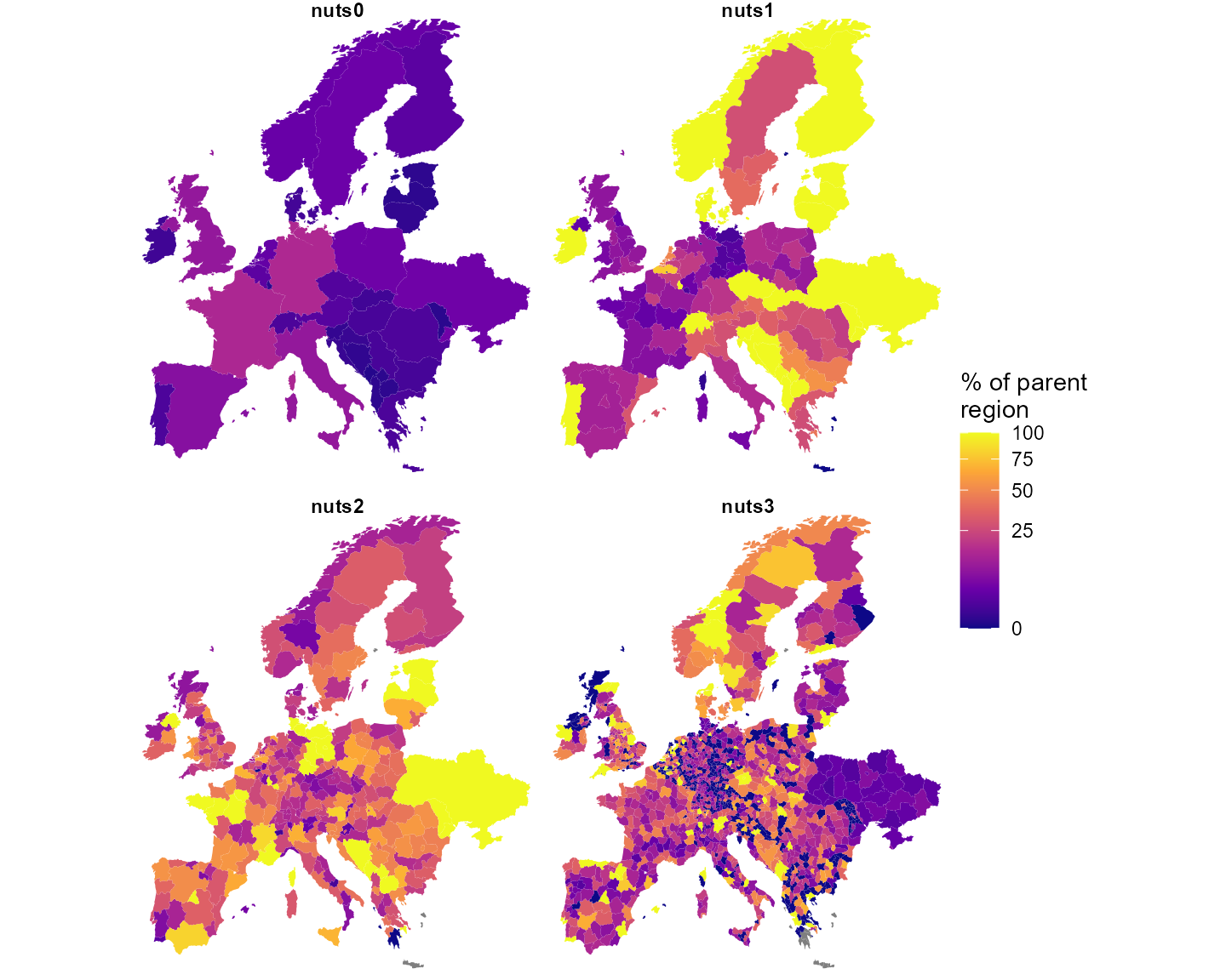

Each region’s share of its parent’s demand, per level. Dark = little of the parent’s demand (including the 442 substation-less regions); grey = the parent itself carries no demand.

Transmission lines

nuts_lines holds every base_s line whose ends fall in different NUTS3 regions. The rest were dropped:

p <- attr(nuts_lines, "reneuro_provenance")
c(lines_total = p$lines_total, intra_nuts3_dropped = p$lines_intra_dropped,
  shipped = nrow(nuts_lines))
#>         lines_total intra_nuts3_dropped             shipped 
#>                7360                4218                3142

57% of lines never leave a NUTS3 region, and they carry 53% of the network’s capacity. The finest level available discards more than half the grid.

Show the aggregation code

centroids <- function(level) {
  s <- level_sf(level)
  cc <- suppressWarnings(sf::st_coordinates(sf::st_centroid(sf::st_geometry(s))))
  tibble(region = s$region, cx = cc[, 1], cy = cc[, 2])
}

haversine <- function(x1, y1, x2, y2) {
  R <- 6371; r <- pi / 180
  a <- sin((y2 - y1) * r / 2)^2 +
       cos(y1 * r) * cos(y2 * r) * sin((x2 - x1) * r / 2)^2
  2 * R * asin(pmin(1, sqrt(a)))
}

agg_lines <- function(level, length_factor = 1.25) {
  m  <- parent_of(level)
  ct <- centroids(level)
  nuts_lines |>
    mutate(f = m[from], t = m[to]) |>
    filter(f != t) |>
    mutate(a = pmin(f, t), b = pmax(f, t)) |>
    left_join(rename(ct, a = region, cx0 = cx, cy0 = cy), by = "a") |>
    left_join(rename(ct, b = region, cx1 = cx, cy1 = cy), by = "b") |>
    mutate(new_len = haversine(cx0, cy0, cx1, cy1) * length_factor,
           lf = if_else(length_km > 0, new_len / length_km, new_len)) |>
    group_by(from = a, to = b) |>
    summarise(s_nom = sum(s_nom), n_lines = n(),
              length_km = first(new_len),
              x = 1 / sum(1 / (lf * x)),        # parallel, length-rescaled
              cx0 = first(cx0), cy0 = first(cy0),
              cx1 = first(cx1), cy1 = first(cy1),
              .groups = "drop")
}

Three rules, taken from pypsa.clustering.spatial:

• s_nom sums — thermal ratings of parallel circuits add;
• length is recomputed as the great-circle distance between the two region centroids times line_length_factor (1.25) — it is not inherited;
• x is rescaled by the length ratio, then parallel-combined as 1 / Σ(1/x).

bind_rows(lapply(LEVELS, function(l) {
  a <- agg_lines(l)
  tibble(level = l, corridors = nrow(a),
         GW = round(sum(a$s_nom) / 1e3),
         median_km = round(median(a$length_km)),
         median_x = round(median(a$x), 2))
}))
#> # A tibble: 4 × 5
#>   level corridors    GW median_km median_x
#>   <chr>     <int> <dbl>     <dbl>    <dbl>
#> 1 nuts0        65   356       459     28.8
#> 2 nuts1       203  1357       253     16.0
#> 3 nuts2       547  2518       154     13.2
#> 4 nuts3      1789  5004        85     11.2

Checked against PyPSA-Eur’s own 41-cluster network, built by its cluster_network rule: the capacity crossing a country boundary sums to 356,352.715 MW there and 356,352.715 MW in the table above. The corridor counts differ (77 against 65) because 41 clusters is not 36 countries. The comparison requires a clone and so is recorded here rather than run.

Aggregating to countries lengthens the network rather than shortening it: a corridor becomes the distance between two national centroids, so r rises and losses are overestimated at coarse levels. Capacity is overestimated for a separate reason: summing thermal ratings ignores N-1 security and loop flows. PyPSA-Eur compensates with a flat s_max_pu = 0.7; the two errors act in opposite directions and do not cancel.

Show code

nets <- bind_rows(lapply(LEVELS, function(l) mutate(agg_lines(l),
                                                    level = l)))
nets$level <- factor(nets$level, levels = LEVELS)

ggplot() +
  geom_sf(data = maps, fill = "wheat", colour = "white", linewidth = 0.1) +
  geom_segment(data = nets,
               aes(x = cx0, y = cy0, xend = cx1, yend = cy1,
                   linewidth = s_nom / 1e3),
               colour = "dodgerblue", alpha = 0.8, lineend = "round") +
  facet_wrap(~level, ncol = 2) +
  scale_linewidth_continuous(range = c(0.1, 1.4), name = "GW") +
  coord_sf(xlim = BOX$xlim, ylim = BOX$ylim, expand = FALSE) +
  theme_void() +
  theme(strip.text = element_text(face = "bold"))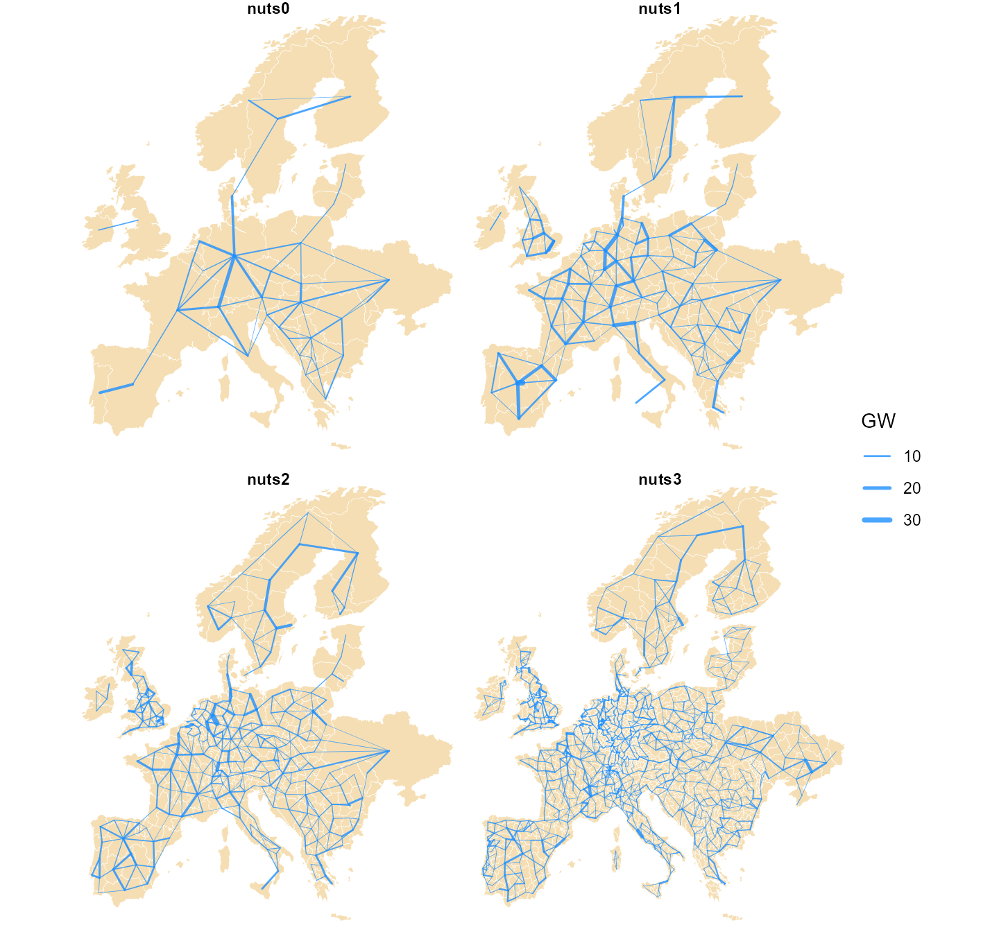

The NUTS-level transmission aggregated to each level: straight chords between region centroids, width proportional to summed thermal rating.

Every quantity and its arithmetic

quantity	kind	fine → coarse	coarse → fine
km2, pop, gdp_total	extensive	sum	split by weight
load_twh, cap_mw, hydro_mw	extensive	sum	split by weight
pot_*	extensive	sum within a carrier	split by weight
n_buses	extensive	sum	cannot be split
gdp (per capita)	intensive	weighted_mean by pop	copy
peak_mw	neither	cannot be derived — recompute from hourly	—
s_nom	extensive	sum, intra-region dropped	—
length	geometric	recomputed from centroids × 1.25	—
x, r	reciprocal	rescale by length, then 1/Σ(1/x)	—
load shape	—	already national; finer adds nothing	—

The kind determines the reduction. Applying the wrong one produces no error: a sum of per-capita GDP, of peaks, or across two overlapping potentials returns a plausible number that does not correspond to any quantity.

9. Known caveats

• Not every upstream dataset covers the whole modeled territory. Some of the redistributable datasets behind the exclusions are unavailable for parts of the PyPSA-Eur domain; where that is the case the affected exclusion is skipped upstream and availability is overstated. The improved layer draws the coverage boundary as a solid red line on the potential maps and applies a flat 0.5 availability derate outside it (non_corine_derate in params.yml) as a conservative stand-in. Extending the coverage with data from other sources is possible — see the source table below and the package’s LICENSE.note for what is used and under which terms.
• Capacity-factor granularity is ~25–30 km. Eligibility is known at 100 m, but the resource is only known per 0.3° cell — a windy ridge and a calm valley inside one cell are indistinguishable. This is the gap the wind-potential layer closes with the 250 m atlas.
• The profiles are one weather year. Potential and variability both come from 2025, and the horizon series reuses those profiles unchanged to 2050. The wind and solar articles take the potential from long-term atlases instead.

10. Sources at a glance

source	licence	vintage	becomes
ERA5 (Copernicus C3S)	CC-BY	2025 hourly	wind / hydro / temperature profiles → weather objects
SARAH-3 (EUMETSAT CM SAF)	CC-BY	2025 hourly	solar profiles → weather objects
Global Wind Atlas (DTU)	CC-BY	v4 long-term	250 m quality bands → the wind-potential layer
Global Solar Atlas (Solargis / World Bank ESMAP)	CC-BY	v2 long-term	~1 km PVOUT → the solar atlas check
ENTSO-E transparency (+ NESO for GB)	open re-use	2025 hourly	national load → demand
powerplantmatching	GPL-3 code, mixed open registries	through 2024	fleet → stock, cap.lo floors, retirement in the horizon series
OpenStreetMap (+ TYNDP projects)	ODbL	2026 extract	grid → trade corridors (the reason the data licence is ODbL)
NUTS / JRC / Eurostat layers	EU open licences	mixed	region geometry + attributes → nuts_gs
Natural Earth (via rnaturalearth)	public domain	1:50m	coastlines and country contours on the figures
technology-data v0.14.0	CC-BY	2020–2050 in 5-year steps	costs → invcost / varom / supply prices

The vintage column carries the split the potential articles turn on: the hourly sources supply variability, the long-term atlases supply the level.

What is not here: the World Database on Protected Areas (non-redistributable; excluded, with the effect documented in LICENSE.note) and the OPSD demand series (replaced by the 2025 ENTSO-E pull).